Send Time Optimization

Did you know that email Send Time Optimization (STO) can improve the open rate by up to 93%? Awesome! Or it might only be 10%. A slightly more credible case study claims that message delivery at the right time resulted in an open rate of 55%, a click rate of 30%, and a conversion rate of 13%. I’ll take that increase any day if there’s a positive ROI. 

Optimization can be applied to any number of problems. It can be applied equally to content, where it may be to the customer’s benefit, as it can be applied to price, where optimization can deliver the maximum possible price for merchants. 

Unfortunately, there’s no way to know in advance what the results of any particular optimization will be without the right data. The only way to get that data is through science!

Science + Data = Profit

Let’s consider the case of email conversion rates. If we’re considering an email message sent to paying customers (we’re not worried about deliverability or the ‘Message From’ text), the factors that can affect customer behavior look like the table below. Think of these five as the variables in an algorithm, where some terms may have an infinite range of possible values, and when we put them all together, we get an impossibly complex set of potential interactions. 

Data like that mentioned above suggests that varying the send time of any particular email message can have a significant impact on the conversion rate, the percentage of customers who open the email and click on the desired call to action link (buy, sell, join, etc.) within the email. How can we determine the best possible time to send an email?

Problem: You and I work at a company that regularly sends email messages to our customers. Our SaaS app allows users to tell us the best time to deliver email messages, but not everyone has taken advantage, particularly our new customers. How can the best time to deliver email messages for users not configured a preference be determined? 

In our case, the best time means “results in the highest conversion rate.” 

N.B. When speaking from our perspective, we refer to “send time.” From the customer’s perspective, we refer to “delivery time.”

Science! 

Have a look at your email app on your phone and desktop. My mobile Gmail account shows six messages before I scroll to see the rest (depending on whether there are message attachments). The desktop version shows 16 messages. Another mobile email app I use shows ten. The desktop web email app for Office 365 shows ten. 

We have an untested assumption that the time an email message is sent/delivered to a customer will impact the conversion rate. In other words, the higher a message is placed in the list of unread messages, the greater the chance of being opened, the critical first step.

If we propose a solution to the STO problem, we want our coworkers to be confident in our recommendations. 

We’ll take our layman’s assumption and cast it as a pair of hypotheses: null and alternative. The null hypothesis is the claim that no relationship exists between two sets of data or variables being analyzed (which we are trying to disprove), and the alternative hypothesis is the hypothesis that we are trying to prove, which is accepted if we have sufficient evidence to reject the null hypothesis.

• Null hypothesis (send time makes no difference): 

There is no relationship between conversion rate and send time.

•  Alternative hypothesis (send time does make a difference): 

The conversion rate varies depending on the time an email is sent.

The conversion rate is the percentage of customers who open the email and click on a call to action link within the email.

The null and alternative hypotheses concern themselves with two variables: 

1. The independent variable is the email send time. 
2. The dependent variable is the conversion rate metric. 

There’s also a third set of variables that, if not carefully controlled, will turn our experiment into rubbish:

• The confounding variables influence the dependent and independent variables, causing a spurious association.

In our case, the confounding variables are the four listed below: 

1. Customer segments
2. Subject line
3. Message content
4. Call to action content.

There could be more confounders like desktop or mobile apps, but the only variables we have control over are these four.

Pro Tip: Use confounding variables likely to have high open, read, and conversion rates, something highly desirable with low friction and free or low cost. While you are making a real offer, our goal is to determine the best send time.

N.B., It is important that none of the confounding variables change during the experiment.

Experiment

We will test our hypothesis using the scientific method or something close to it. Our starting point is the independent variable: when should we send the messages during the experiment? We have two ways to tackle this problem: use our intuition or use our data.

As mentioned previously, our SaaS app allows users to set a preference for email delivery time. If we query the preference data using the user’s local time, we will get something like the normal distribution:

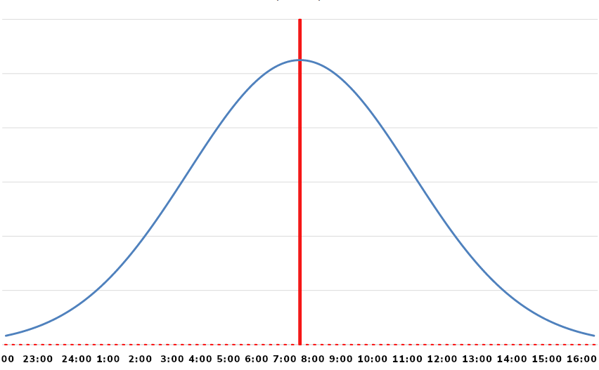
                     Fig. 1 Normal distribution of preferred email delivery times; median: 0730 local. 

According to users with a preference, the median time for delivery is 7:30-ish. It’s unfortunate that there’s such a broad range of preferred times; five hours is a big window. Ideally, we want to send the messages one hour apart. Having a five-hour window means five customer segments with at least 1,000 each. 

The choice of how many independent variables (send times) to test boils down to the number of new customers that can participate in the experiment. In this case, we’re a global company with about 30,000 new customers per month, and it usually takes a full month before half of them choose a preferred time. That leaves us with 15,000 spread out across the world, with about half of those in the United States. 7,000 is enough to test three independent variables. Ideally, the minimum number of customers is 1,000, so we can be fairly confident in the experiment’s results.

N.B. All times are local.

We will send the messages three times: t1, t2, and t3.

Where:

1. t1 is the initial email send time: 0500 local (two and a half hours before the peak time of 0730) local.
2. t2 is two hours after t1.
3. t3 is two hours after t2.

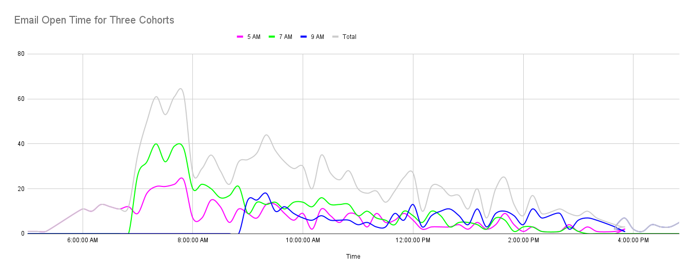
                                     Fig. 2 Three cohorts, each with a two-hour window. 

This will give us a delivery time window of six hours, covering a large portion of the normal distribution of our existing customers. As the US covers six time zones, we’ll have to do a bit of time arithmetic to arrive at the correct data center or cloud send-time for each customer in each cohort so that the messages are sent at the correct local time. 

!Important: Do not spread out the send times within the cohort’s time window; try to send all messages so that they are delivered as close as possible to each of the three times, t1, t2, and t3.

Customer Segmentation, AKA Cohort Engineering

We should consider a few other criteria when creating the customer cohorts. Our previous work on demographics shows that 90% of our customers live in metropolitan areas. We can use zip codes or geolocation to create the location predicate and split each metro into three groups. Are there any other criteria that might be useful? 

• Mobile vs. desktop users
• Android vs iOS
• Windows vs Mac
• User-agent
• Organization size
• SaaS subscription plan

I’ll leave it to you to decide how to slice and dice, but keep in mind that if you can, use whatever demo- or psychographic data you have and ensure that each of the three segments is well-balanced. That will avoid trouble when we want to do some analytic exploration with the results.

Launch in 3, 2, HOLD THE LAUNCH! 

Before we start sending messages, we need to be sure we have the right observability in place. We need to know more than a few of the key events like message-was-opened and message-is-converted. We must also know when anything goes wrong, anywhere in the customer/experiment journey. We must also be alerted if certain failure conditions are met so we can stop the experiment before wasting the very real offer we want our real customers to accept. Be sure to include the actual send time.

Another group of facts that may come in handy at some point is the network and geolocation data. Perhaps a significant number of customers open messages while online for coffee or

When everything is ready, all that’s left to do is push the big, red GO! Button and collect the data. How long should you wait?

Data Exploration and Analysis

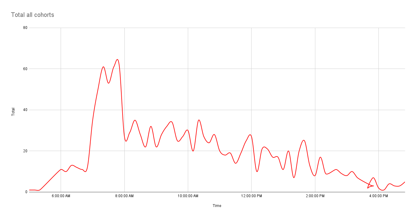
As you can see from the three graphs, the results have dropped to a trickle within 48 hours of beginning the experiment. This information, too, is highly valuable. It’s safe to assume that each customer receives more messages as time passes, pushing the experimental message further down the list. This is where tracking each user’s app or user-agent will allow you to correlate email app window size with message open rate.

In addition to looking at each cohort individually, look at all three combined to see if all patterns are common. For example, maybe all of the tracked customer rates (open, clicked web page link, clicked call to action link) will decline just before lunch and remain low until the end of the day.

Other patterns may be related to subscription plans or the customer’s phone model. Perhaps iPhone users are busy getting a double soy chai latte in the 15 minutes before they start their day, and that’s when they check their email apps most thoroughly.

Finally, it may be that regardless of when the emails were sent, there is a definite peak in opening emails around 8:30 a.m. local time or 8:00 or 9:00. YMMV.

Results

Finally, the results are in, and you have an unambiguous result. You can clearly see that new customers have a preference for reading email at 8:24 a.m. From this day forward, you can set the default email send time for new customers to this time. Hooray!

All left to do now is write up a paper, distribute it to your coworkers, and get approval to change the default send time unless one of the business unit heads or product owners wants a meeting to discuss the results –all the results – including the analytic explorations and assumptions. Assumptions? 

Discussion/Assumptions

We all make assumptions, or so I assume. I’ve never seen any research on this question. Before you write your conclusion and send out the paper, now would be a good time to think about any assumptions made and include them in a discussion section. As an example, in preparing the cohorts, we tried to balance, as much as possible, all of the definitive customer attributes that we know about, like subscription plan, company size, and so on. However, we know that company culture can vary quite a bit. Some companies – perhaps most of them – may have fully adopted work-from-home.

STO With Deep Learning 

Suppose the results of your experiment do not show a strong enough signal across each or all cohorts.  Or, perhaps while you were exploring the experiment’s result data, you noticed a strong signal from customers in Los Angeles using their iPhones. They would like to check their email later in the morning –maybe after a run on the beach or while sitting in traffic on the 405.

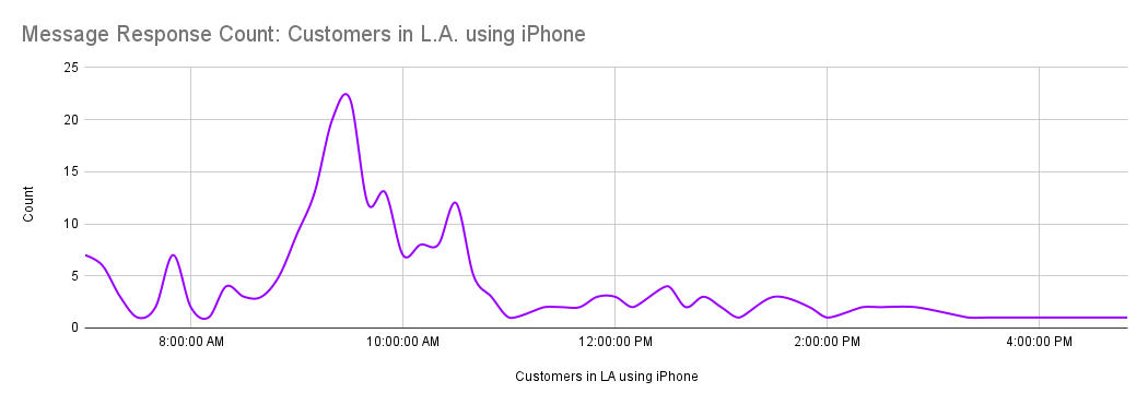
You then look at your data from existing customers who have expressed a preference, also from LA, and also using their iPhone. This group also strongly prefers receiving emails between 9 and 10 am. Perhaps there are other strong correlations like this in your customer db –if so, you might be able to train a machine learning model to predict the best time to send emails to new users. How would you do this when you’ve never done ML training before? Is it even possible? 

Of course it is! Like most mid- to senior-level programmers, I have won so many battles with tough problems that I believe I can do just about anything with code. So, let’s give it a shot. Even if your org’s data set doesn’t lend itself to training an ML model, you will gain important insights into the hard work our data science and engineering colleagues do, understand just how difficult we make their job by sending them lousy data, and you’ll learn some important concepts and vocabulary that will become a larger part of every programmer’s job description in the coming years. 

Two Methods: Supervised or Unsupervised Learning

The core of the problem is prediction: which ten or 15-minute send time slot are new users most likely to choose? This problem can be addressed by two classes of ML models: supervised and unsupervised learning. It may turn out that the best path for you is to use unsupervised clustering to explore and understand your data and help you hunt for similarities (clusters) in your data. If so, you can use clustering to predict send times. Or you can continue to try the supervised learning path. What’s the key difference? As far as you’re concerned, supervised learning requires labeled data, and unsupervised data does not, so unsupervised learning is a little easier. Fortunately, if your customer data includes their preferred email send time (or equivalent for your use case), then you're halfway to having labeled data.

Supervised Learning With XGBoost

XGBoost is an excellent choice for this problem. There are numerous Python and R implementation tutorials directly related to our problem. It doesn’t require massive computing resources, and it doesn’t require optimization of the parameters or tuning. Perfect for beginners like you and me.

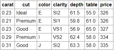
I don’t have the space in this article to walk you through each step, but I highly recommend the following tutorial in Python: Using XGBoost in Python. The tutorial is centered around the problem of predicting (classifying) diamond prices. Running through the tut shouldn’t take you more than an hour. How are diamond prices like customer’s preferred email delivery times? Actually, the business or data domain makes little difference to the ML model. 

Diamond Data 

Customer Data

In both cases, the domain is not important to the problem. We have a bunch of data fields; some are relevant to the problem, some perhaps not. With the diamond data, we want to predict the price, while in the customer data, we want to predict the preferred send time. Yes, you and I know that there is a calculation that can be made using diamond data attributes, but the ML model doesn’t know that and doesn’t need to know that to achieve a reliable price prediction. 

The answers are in the data - or not.

What is important are the attributes in the data. Do you have enough attributes/fields/columns in your customer data to answer a basic question: is a given new customer’s data similar enough to any existing groups of customers such that the new user would likely choose the existing user email send time? Our second ML model may help you answer that question.

After working through the XGBoost tutorial, try the same with your data. You will likely have to iterate over a number of variations of the data you use. If that’s not working out well, move on to clustering.

Unsupervised Learning With *–Clustering

What is clustering? Datacamp.com has a very good introduction to clustering. 

 “Clustering is an unsupervised machine learning technique with many applications in pattern recognition, image analysis, customer analytics, market segmentation, social network analysis…

... it is an iterative process of information discovery that requires domain expertise and human judgment used frequently to make adjustments to the data and the model parameters to achieve the desired result. ”

Basically, your clustering model’s chosen algorithm processes your data and produces a result set of two-dimensional vectors: X and Y coordinates for each record in the data. These can be presented as a table or as a visualization like this, where it’s much easier to see the clusters:

For now, start with K-means clustering, a widely used algorithm for clustering tasks due to its use of intuition and ease of implementation. It is a centroid-based algorithm where the user must define the number of clusters it wants to create. The number of clusters in our case is the number of send time slots we want predictions for, e.g., from 7 am to 10 am every 15 minutes, so 12 clusters (K = 12).

Again, I highly recommend starting with a tutorial and then moving on to your customer data. I can highly recommend this tut from Kaggle: Customer-Segmentation with k-means.

Once you’re ready to use your data, the overall workflow goes like this:

1. Explore your data and try to intuitively identify features that might show a correlation with the existing user’s preferred send times. You will probably have too much data for existing and no preference.

2. Iterate over the attributes/columns/fields until some clustering appears.

3. Refine until you have enough clusters to cover a large portion of preferred send times.

4. If your data shows absolutely no clustering correlated with send times, you have two options:

   1. Try to identify and collect data that would help to discern a preference or

   2. Accept defeat gracefully; sometimes, the null hypothesis wins.

5. If any of your datasets shows clusters correlated to send times, you have won the golden ticket!

6. Next, you must derive the cluster centroids (find a real or synthetic vector at the center of each send-time cluster).

7. Collect a dataset of new users who have not expressed a send time preference. For each of the new users, calculate their vectors using the same method used to create the cluster vectors.

8. Measure the difference (cosine similarity or Euclidean distance) between each user’s vector from #7 to each cluster centroid, and the centroid with the smallest difference is your new optimal send time.

9. Over the next few weeks, check that set of new users to see if their preferred send time matches the predicted time.

10. You can also test this method against a set of existing user data with preferred send times.

11. If, by some miracle, this all works out very nicely, then you have won the golden ticket!

12. Try another experiment; only this time, send out a new experimental email message using the predicted email send time and see if the conversion rate is higher than during the first experiment.

Conclusion

If you did some research online on this topic, you probably noticed that there are a lot of companies that make it their business to provide a solution to this problem; it’s worth a lot of money to those who can solve it or increase the conversion rate enough to justify the expense.

In addition to the economic benefit you could potentially deliver to your organization, you will be able to add a new and important section to your CV: created and conducted data science experiments in the area of message send time optimization that resulted in a 27% increase in conversion rate and increased ARR by 4%.

Now, that is something worth working toward. Good luck!