Efficiently Processing Billions of Rows Daily With Presto
In this article, we will delve into strategies for efficiently storing and processing large datasets using Presto.
Join the DZone community and get the full member experience.
Join For FreeIn a world where companies rely heavily on data for insights about their performance, potential issues, and areas for improvement, logging comprehensively is crucial, but it comes at a cost. If not stored properly it can become cumbersome to maintain, query, and overall expensive.
Logging detailed user activities like time spent on various apps, which interface where they are active, navigation path, app start-up times, crash reports, country of login, etc. could be vital in understanding user behaviors — but we can easily end up with billions of rows of data, which can quickly become an issue if scalable solutions are not implemented at the time of logging.
In this article, we will discuss how we can efficiently store data in an HDFS system and use some of Presto’s functionality to query massive datasets with ease, reducing compute costs drastically in data pipelines.
Partitioning
Partitioning is a technique where similar logical data can be clubbed together and stored in a single file making retrieval quicker. For example, let's consider an app like YouTube. It would be useful to group data belonging to the same date and country into one file, which would result in multiple smaller files making scanning easier. Just by looking at the metadata, Presto can figure out which one of the specific files needs to be scanned based on the query the user provides.
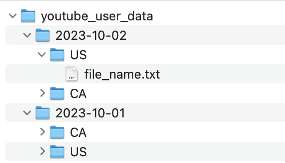
Internally, a folder called youtube_user_data would be created within which multiple subfolders would be created for each partition by date and country (e.g., date=2023-10-01/country=US). If the app was launched in 2 countries and has been active for 2 days, then the number of files generated would be 2*2 = 4 (cartesian product of the unique values in the partition columns).
Hence, choosing columns with low cardinality is essential. For example, if we add interface as another partition column, with three possible values (ios, android, desktop), it would increase the number of files to 2×2×3=12.

Based on the partitioning strategy described, the data would be stored in a directory structure like this:

Below is an example query on how to create a table with partition columns as date and country:
CREATE TABLE youtube_user_data (
  user_id BIGINT,
  Age int,
  Video_id BIGINT,
  login_unixtime BIGINT,
  interface VARCHAR,
  ip_address VARCHAR,
  login_date VARCHAR,
  country VARCHAR
    …
    …
)
WITH (
  partitioned_by = ARRAY[‘login_date’, ‘country’],
  format = 'DWRF',
  oncall = ‘your_oncall_name’,
  retention_days = 60,
);
Ad Hoc Querying
When querying a partitioned table, specifying only the needed partitions can speed up your query wall time greatly.
SELECT
    SUM(1) AS total_users_above_30
FROM youtube_user_data
WHERE
    Login_date = ‘2023-10-01’
    And country = ‘US’
    And age > 30
By specifying the partition columns as filters in the query, Presto will directly jump to the folder 2023-10-01 and US, and retrieve only the file within that folder skipping the scanning of other files completely.
Scheduling Jobs
If the source table is partitioned by country, then setting up daily ETL jobs also becomes easier, as we can now run them in parallel. For example:
# Sample Dataswarm job scheduling, that does parallel processing
# taking advantage of partitions in the source table
insert_task = {}
wait_for = {}

for country in ["US", "CA"]:
   # wait for job
   wait_for[country] = WaitforOperator(
       table="youtube_user_data",
       partitions=f"login_date=<DATEID>/country={country}"
   )

   # insert job
   insert_task[country] = PrestoOperator(
       dep_list = [wait_for[country]],
       input_data = { "in": input.table("youtube_user_data").col("login_date").eq("<DATEID>")
                      .col("country").eq(country)},
       output_data = {"out": output.table("output_table_name").col("login_date").eq("<DATEID>")
                      .col("country").eq(country)},
       select = """
           SELECT
               user_id,
               SUM(1) as total_count
           FROM <in:youtube_user_data>
       """
)- Note: The above uses Dataswarm as an example for processing/inserting data.
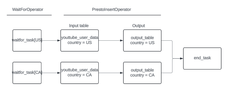
Here, there will be two parallel running tasks — insert_task[US] and insert_task[CA] — which will query only the data pertaining to those partitions and load them into a target table which would also be partitioned on country and date. Another benefit is that waitforoperator can be set up to check if that particular partition of interest has landed rather than waiting for the whole table. If, say, CA data is delayed, but US data has landed, then we can start the US insert task first and later once CA upstream data lands, then kick off the CA insert job.

Above is a simple DAG showing the sequence of events that would be run.
Bucketing
If frequent Group by and join operations are to be performed on a table, then we can further optimize the storage using bucketing. Bucketing organizes data into smaller chunks within a file based on a key column (e.g., userid), so when querying, Presto would know in which bucket a specific ID would be present.
How to Implement Bucketing
- Choose a bucketing column: Pick a key column that is commonly used for
joinsandgroup bys. - Define buckets: Specify the number of buckets to divide the data into.
CREATE TABLE youtube_user_data (
  user_id BIGINT,
  Age int,
  Video_id BIGINT,
  login_unixtime BIGINT,
  interface VARCHAR,
  ip_address VARCHAR,
  login_date VARCHAR,
  country VARCHAR
    …
    …
)
WITH (
  partitioned_by = ARRAY[‘login_date’, ‘country’],
  format = 'DWRF',
  oncall = ‘your_oncall_name’,
  retention_days = 60,
  bucket_count = 1024,
  bucketed_by = ARRAY['user_id'],
);- Note: The bucket size should be a power of 2. In the above example, we chose 1024 (2^10).
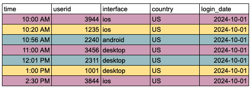
Before Bucketing
Data for a partition is stored in a single file, requiring a full scan to locate a specific user_id:

After Bucketing
Userids are put into smaller buckets based on which range they fall under.

You'll notice that user IDs are assigned to specific buckets based on their value. For example, a new user ID of 1567 would be placed in Bucket 1:
- Bucket 1: 1000 to 1999
- Bucket 2: 2000 to 2999
- Bucket 3: 3000 to 3999
- Etc.
When performing a join with another table — say, to retrieve user attributes like gender and birthdate for a particular user (e.g., 4592) — it would be much quicker, as Presto would know under which bucket (bucket 4) that user would be so it can directly jump to that specific one and skip scanning the others.
It would still need to search where that user would be within that bucket. We can speed up that process as well by taking advantage of sorting the data on the key ID while storing them within each of the buckets, which we will explore in the later section.
SELECT
    a.user_id,
    b.gender,
    b.birthdate
FROM youtube_user_data a
JOIN dim_user_info b
    ON a.user_id = b.user_id
WHERE
    a.login_date = '<DATEID>'
    AND a.country = 'US'
    AND b.date = '<DATEID>'
Hidden $bucket Column
For bucketed tables, there is a hidden column to let you specify the buckets you want to read data from. For example, the following query will count over bucket #17 (the bucket ID starts from 0).
SELECT
	SUM(1) AS total_count
FROM youtube_user_data
WHERE
 	ds='2023-05-01'
 	AND "$bucket" = 17
The following query will roughly count over 10% of the data for a table with 1024 buckets:
SELECT
	SUM(1) AS total_count
FROM youtube_user_data
WHERE
	ds='2023-05-01'
	AND "$bucket" BETWEEN 0 AND 100
Sorting
To further optimize the buckets, we can sort them while inserting the data so query speeds can be further improved, as Presto can directly jump to the specific index within a specific bucket within a specific partition to fetch the data needed.
How to Enable Sorting
- Choose a sorting column: Typically, this is the same column used for bucketing, such as
user_id. - Sort data during insertion: Ensure that data is sorted as it is inserted into each bucket.
CREATE TABLE youtube_user_data (
  user_id BIGINT,
  Age int,
  Video_id BIGINT,
  login_unixtime BIGINT,
  interface VARCHAR,
  ip_address VARCHAR,
  login_date VARCHAR,
  country VARCHAR
    …
    …
)
WITH (
  partitioned_by = ARRAY[‘login_date’, ‘country’],
  format = 'DWRF',
  oncall = ‘your_oncall_name’,
  retention_days = 60,
  bucket_count = 1024,
  bucketed_by = ARRAY['user_id'],
  sorted_by = ARRAY['userid']
);
In a sorted bucket, the userids are inserted in an orderly manner, which makes retrieval efficient. It becomes very handy when we have to join large tables or perform aggregations across billions of rows of data.
Conclusion
- Partitioning: For large datasets, partition the table on low cardinality columns like
date,country, andinterface, which would result in smaller HDFS files. Presto can then only query the needed files by looking up the metadata/file name. - Bucketing and sorting: If a table is to be used frequently in several
joinorgroup bys, then it would be beneficial to bucket and sort the data within each partition further reducing key lookup time. - Caveat: There is an initial compute cost for bucketing and sorting as Presto would have to remember the order of the key while inserting. However, this one-time cost could be justified by savings in repeated downstream queries.
Opinions expressed by DZone contributors are their own.

Comments