Probabilistic Graphical Models: A Gentle Introduction

Definition: "Probabilistic graphical models (PGM) is a technique of compactly representing a joint distribution by exploiting dependencies between the random variables. " [4].

This definition might seem complex at first but it can be clarified by breaking down the core elements of PGMs:

Model

A model is a formal representation of a system or process, capturing its essential features and relationships. In the context of PGMs, the model comprises variables that represent different aspects of the system and the probabilistic relationships among them. This representation is independent of any specific algorithm or computational method used to process the model. Models can be developed using various techniques:

• Learning from data: Statistical and machine learning methods can be employed to infer the structure and parameters of the model from historical data.
• Expert knowledge: Human experts can provide insights into the system, which can be encoded into the model.
• Combination of both: Often, models are constructed using a mix of data-driven approaches and expert knowledge.

Algorithms are then used to analyze the model, answer queries, or perform tasks based on this representation.

Probabilistic

PGMs handle uncertainty by explicitly incorporating probabilistic principles. Uncertainty in these models can stem from several sources:

• Noisy data: Real-world data often includes errors and variability that introduce noise into the observations.
• Incomplete knowledge: We may not have access to all relevant information about a system, leading to partial understanding and predictions.
• Model limitations: Models are simplifications of reality and cannot capture every detail perfectly. Assumptions and simplifications can introduce uncertainty.
• Stochastic nature: Many systems exhibit inherent randomness and variability, which must be modeled probabilistically.

Graphical

The term "graphical" refers to the use of graphs to represent complex systems. In PGMs, graphs are used as a visual and computational tool to manage the relationships between variables:

• Nodes: Represent random variables or their states
• Edges: Represent dependencies or relationships between variables

Graphs provide a compact and intuitive way to capture and analyze the dependencies among a large number of variables. This graphical representation allows for efficient computation and visualization, making it easier to work with complex systems.

Preliminary Concepts

Learning, Inference, and Sampling

PGMs are powerful for exploring and understanding complex domains. Their utility lies in three key operations[1]: 

• Learning: This entails estimating the parameters of the probability distribution from data. This process allows the model to generalize from observed data and make predictions about unseen data.
• Inference: Inference is the process of answering queries about the model, typically in the form of conditional distributions. It involves determining the probability of certain outcomes given observed variables, which is crucial for decision-making and understanding dependencies within the model.
• Sampling: Sampling refers to the ability to draw samples from the probability distribution defined by the graphical model. This is important for tasks like simulation, approximation, and exploring the distribution's properties, and is also often used in approximate inference methods when exact inference is computationally infeasible.

Factors in PGMs

In PGMs, a factor is a fundamental concept used to represent and manipulate the relationships between random variables. A factor is a mathematical construct that assigns a value to each possible combination of values for a subset of random variables. This value could represent probabilities, potentials, or other numerical measures, depending on the context. The scope of a factor is the set of variables it depends on. 

Types of Factors

• Joint distribution: Represents the full joint probability distribution over all variables in the scope
• Conditional Probability Distribution (CPD): Provides the probability of one variable given the values of others; It is often represented as a table, where each entry corresponds to a conditional probability value.
• Potential function: In the context of Markov Random Fields, factors represent potential functions, which assign values to combinations of variables but may not necessarily be probabilities.

Operations on Factors

• Factor product: Combines two factors by multiplying their values, resulting in a new factor that encompasses the union of their scopes
• Factor marginalization: Reduces the scope of a factor by summing out (marginalizing over) some variables, yielding a factor with a smaller scope
• Factor reduction: Focuses on a subset of the factor by setting specific values for certain variables, resulting in a reduced factor

Factors are crucial in PGMs for defining and computing high-dimensional probability distributions, as they allow for efficient representation and manipulation of complex probabilistic relationships.

Representation in PGMs

Representation of PGMs involves two components:

• Graphical structure that encodes dependencies among variables
• Probability distributions or factors that define the quantitative relationships between these variables

The choice of representation affects both the expressiveness of the model and the computational efficiency of inference and learning.

Bayesian Networks

A Bayesian network is used to represent causal relationships between variables. It consists of a directed acyclic graph (DAG) and a set of Conditional Probability Distributions (CPDs) associated with each of the random variables [4]. 

Key Concepts in Bayesian Networks

• Nodes and edges: Nodes represent random variables, and directed edges represent conditional dependencies between these variables. An edge from node A to node B indicates that A is a parent of B i.e. B is conditionally dependent on A.
• Acyclic nature: The graph is acyclic, meaning there are no cycles, ensuring that the model represents a valid probability distribution.
• Conditional Probability Distributions (CPDs): In a Bayesian Network, each node Xi has an associated Conditional Probability Distribution (CPD) that defines the probability of Xi given its parents in the graph. These CPDs quantify how each variable depends on its parent variables. The overall joint probability distribution can then be decomposed into a product of these local CPDs.
• Conditional independence: The structure of the graph encodes conditional independence assumptions. Specifically, a node is Xi conditionally independent of its non-descendants given its parents. This assumption allows for the decomposition of the joint probability distribution into a product of conditional distributions. This factorization allows the complex joint distribution to be efficiently represented and computed by leveraging the network's graphical structure.

Common Structures in Bayesian Networks

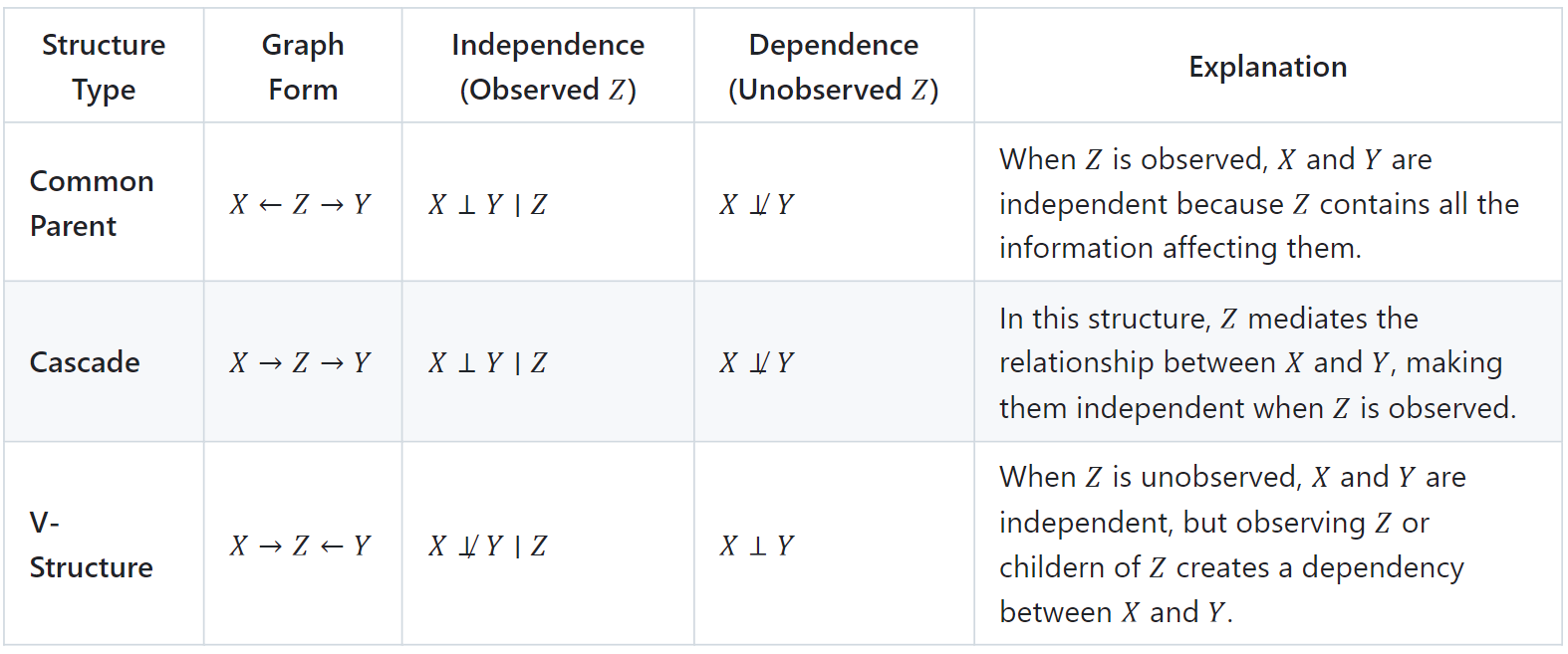
To better grasp how a Directed Acyclic Graph (DAG) captures dependencies between variables, it's essential to understand some of the common structural patterns in Bayesian networks. These patterns influence how variables are conditionally independent or dependent, shaping the flow of information within the model. By identifying these structures, we can gain insights into the network's behavior and make more efficient inferences. The following table summarizes common structures in Bayesian networks and explains how they influence the conditional independence or dependence of variables [5, 6]:

Example

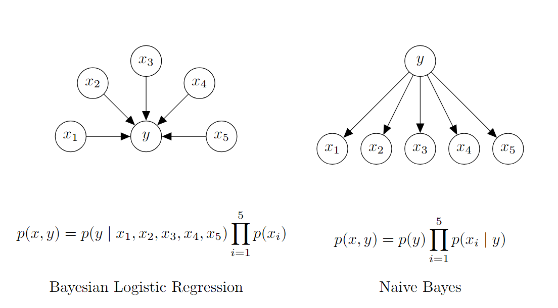
As a motivating example, consider an email spam classification model where each feature, Xi, encodes whether a particular word is present, and the target, y, indicates whether the email is spam. To classify an email, we need to compute the joint probability distribution, P(Xi,y), which models the relationship between the features (words) and the target (spam status).

Figure 1 (below) illustrates two Bayesian network representations for this classification task. The network on the left represents Bayesian Logistic Regression, which models the relationship between the features and y in the most general form. This model captures potential dependencies between words and how they collectively influence the probability that an email is spam.

In contrast, the network on the right shows the Naive Bayes Model, which simplifies the problem by making a key assumption: the presence of each word in an email is conditionally independent of the presence of other words, given whether the email is spam or not. This conditional independence assumption reduces the model's complexity, as it requires far fewer parameters than a fully general model like Bayesian logistic regression.

Dynamic Bayesian Network (DBN)

A Dynamic Bayesian Network (DBN) is an extension of a Bayesian network that models sequences of variables over time. DBNs are particularly useful for representing temporal processes, where the state of a system evolves over time. A DBN consists of the following components:

• Time slices: Each time slice represents the state of the system at a specific point in time. Nodes in a time slice represent variables at that time and edges within the slice capture dependencies at that same time.
• Temporal dependencies: Edges between nodes in successive time slices represent temporal dependencies, showing how the state of the system at one time step influences the state at the next time step. These dependencies allow the DBN to capture the dynamics of the system as it progresses through time. 

DBNs combine intra-temporal dependencies (within a time slice) and inter-temporal dependencies (across time slices), allowing them to model complex temporal behaviors effectively. This dual structure is useful in applications like speech recognition, bioinformatics, and finance, where past states strongly influence future outcomes. In DBNs, we often make use of the Markov assumption and time invariance to simplify the model's complexity while maintaining its predictive power.

• Markov assumption simplifies the DBN by assuming that the state of the system at time t + 1 depends only on the state at time t, ignoring any earlier states. This assumption reduces the complexity of the model by focusing only on the most recent state, making it computationally more feasible.
• Time invariance implies that the dependencies between variables and the conditional probability distributions remain consistent across time slices. This means that the structure of the DBN and the parameters associated with each conditional distribution do not change over time. This assumption greatly reduces the number of parameters that need to be learned, making the DBN more tractable.

DBN Structure

A dynamic Bayesian network (DBN) is represented by a combination of two Bayesian networks:

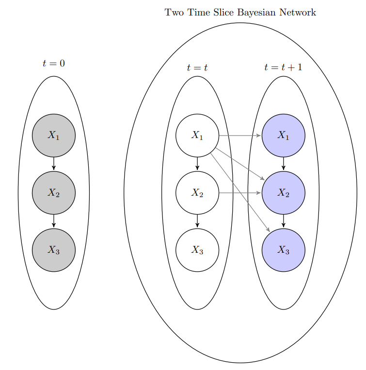
• Initial Bayesian Network (BN0) over the initial state variables which models the dependencies among the variables at the initial time slice (time 0). This network specifies the distribution over the initial states of the system.
• Two-Time-Slice Bayesian Network (2TBN), which models the dependencies between the variables in two consecutive time slices. This network models the transition dynamics from time t to time t+1, encoding how the state of the system evolves from one-time step to the next.

Example: Consider a DBN where the states of three variables (X1,X2,X3). This structure highlights both intra-temporal and inter-temporal dependencies and the relationships between the variables across different time slices, as well as the dependencies within the initial time slice.

Hidden Markov Models

A Hidden Markov Model (HMM) is a simpler special case of a DBN and is widely used in various fields such as speech recognition, bioinformatics, and finance. While DBNs can model complex relationships among multiple variables, HMMs focus specifically on scenarios where the system can be represented by a single hidden state variable that evolves over time. 

Markov Chain Foundation

Before delving deeper into HMMs, it is essential to understand the concept of a Markov Chain, which forms the foundation for HMMs. A Markov Chain is a mathematical model that describes a system that transitions from one state to another in a chain-like process. It is characterized by the following properties [7]:

• States: The system is in one of a finite set of states at any given time.
• Transition probabilities: The probability of transitioning from one state to another is determined by a set of transition probabilities.
• Initial state distribution: The probabilities associated with starting in each possible state at the initial time step.
• Markov property: The future state of the system depends only on the current state and not on the sequence of states that preceded it.

A Hidden Markov Model (HMM) extends the concept of a Markov Chain by incorporating hidden states and observable emissions. While Markov Chains directly model the transitions between states, HMMs are designed to handle situations where the states themselves are not directly observable, but instead, we observe some output that is probabilistically related to these states.

The key components of an HMM include:

• States: The different conditions or configurations that the system can be in at any given time. Unlike in a Markov Chain, these states are hidden, meaning they are not directly observable.
• Observations: Each state generates an observation according to a probability distribution. These observations are the visible outputs that we can measure and use to infer the hidden states.
• Transition probabilities: The probability of moving from one state to another between consecutive time steps. These probabilities capture the temporal dynamics of the system, similar to those in a Markov Chain.
• Emission probabilities: The probability of observing a particular observation given the current hidden state. This links the hidden states to the observable data, providing a mechanism to relate the underlying system behavior to the observed data.
• Initial state distribution: The probabilities associated with starting in each possible hidden state at the initial time step.

An HMM can be visualized as a simplified version of a DBN with one hidden state variable and observable emissions at each time step. In essence, an HMM is designed to handle situations where the states of the system are hidden, but the observable data provides indirect information about the underlying process. This makes HMMs powerful tools for tasks like speech recognition, where the goal is to infer the most likely sequence of hidden states (e.g., phonemes) from a sequence of observed data (e.g., audio signals).

Markov Networks

While Bayesian Networks are directed graphical models used to represent causal relationships, Markov Networks, also known as Markov Random Fields, are undirected probabilistic graphical models. They are particularly useful when relationships between variables are symmetric or when cycles are present, as opposed to the acyclic structure required by Bayesian Networks. Markov Networks are ideal for modeling systems with mutual interactions between variables, making them popular in applications such as image processing, social networks, and spatial statistics.

Key Concepts in Markov Networks [5,6]

Undirected Graphical Structure

In a Markov network, the relationships between random variables are represented by an undirected graph. Each node represents a random variable, while each edge represents a direct dependency or interaction between the connected variables. Since the edges are undirected, they imply that the relationship between the variables is symmetric — unlike Bayesian networks, where the edges indicate directed conditional dependencies.

Factors and Potentials

Instead of using Conditional Probability Distributions (CPDs) like Bayesian networks, Markov networks rely on factors or potential functions to describe the relationships between variables. A factor is a function that assigns a non-negative real number to each possible configuration of the variables involved. These factors quantify the degree of compatibility between different states of the variables within a local neighborhood or clique in the graph.

Cliques in Markov Networks

A clique is a subset of nodes in the graph that are fully connected. Cliques capture the local dependencies among variables. This means that within a clique, the variables are not independent and their joint distribution cannot be factored further. In Markov networks, potential functions are defined over cliques, capturing the joint compatibility of the variables in these fully connected subsets. The simplest cliques are pairwise cliques (two connected nodes), but larger cliques can also be defined in more complex Markov networks.

Markov Properties

The graph structure of a Markov network encodes various Markov properties, which dictate the conditional independence relationships among the variables:

• Pairwise Markov Property: Two non-adjacent variables are conditionally independent given all other variables. Formally, for nodes X and Y, if they are not connected by an edge, they are conditionally independent given the rest of the nodes.
• Local Markov Property: A variable is conditionally independent of all other variables in the graph given its neighbors (the variables directly connected to it by an edge). This reflects the idea that the dependency structure of a variable is fully determined by its local neighborhood in the graph. 
• Global Markov Property: Any two sets of variables are conditionally independent given a separating set. If a set of nodes separates two other sets of nodes in the graph, then the two sets are conditionally independent given the separating set.

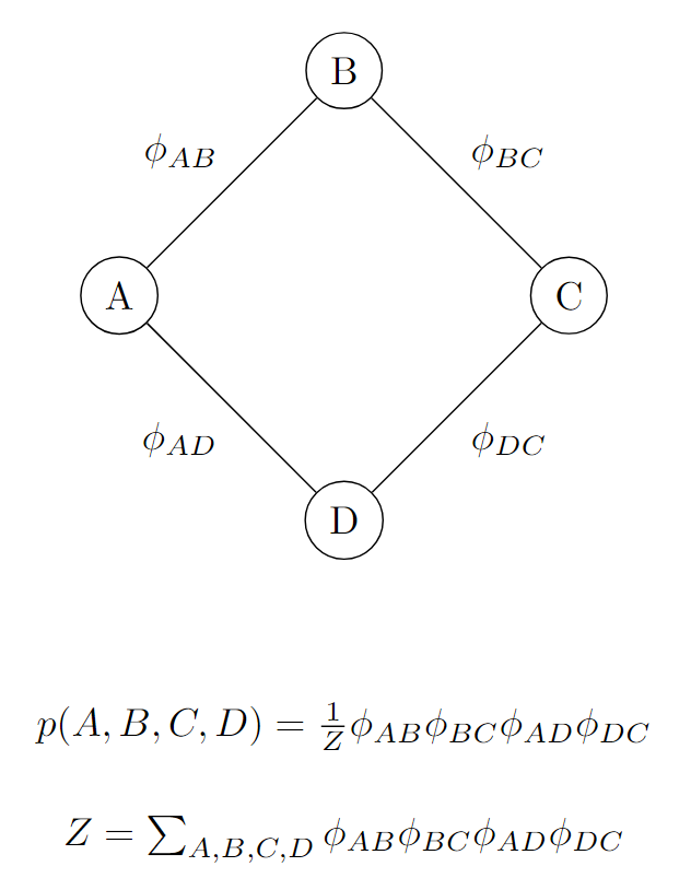
Example: Consider the Markov network field as illustrated in Figure 4. The network consists of four variables, A, B, C, and D, represented by the nodes. The edges between these nodes are labeled with factors ϕ. These factors represent the level of association or dependency between each pair of connected variables. The joint probability distribution over all variables A, B, C, and D is computed as the product of all the pairwise factors in the network, along with a normalizing constant Z, which ensures the probability distribution is valid (i.e., sums to 1). 

Learning and Inference 

Inference and learning are two critical components of PGMs, which will be explored in a follow-up article.

Conclusion

Probabilistic graphical models represent probability distributions and capture conditional independence structures using graphs. This allows the application of graph-based algorithms for both learning and inference. Bayesian Networks are particularly useful for scenarios involving directed, acyclic dependencies, such as causal reasoning. Markov Networks provide an alternative, especially suited for undirected, symmetric dependencies common in image and spatial data. These models can perform learning, inference, and decision-making in uncertain environments, and find applications in a wide range of fields such as healthcare, natural language processing, computer vision, and financial modeling.

References

1. Shrivastava, H. and Chajewska, U., 2023, September. Neural graphical models. In European Conference on Symbolic and Quantitative Approaches with Uncertainty (pp. 284-307). Cham: Springer Nature Switzerland.
2. Kapteyn, M.G., Pretorius, J.V. and Willcox, K.E., 2021. A probabilistic graphical model foundation for enabling predictive digital twins at scale. Nature Computational Science, 1(5), pp.337-347.
3. Louizos, C., Shalit, U., Mooij, J.M., Sontag, D., Zemel, R. and Welling, M., 2017. Causal effect inference with deep latent-variable models. Advances in neural information processing systems, 30.
4. Ankan, A. and Panda, A., 2015, July. pgmpy: Probabilistic Graphical Models using Python. In SciPy (pp. 6-11).
5. Koller, D., n.d. *Probabilistic graphical models* [Online course]. Coursera. Available at: <https://www.coursera.org/learn/probabilistic-graphical-models?specialization=probabilistic-graphical-models> (Accessed: 9 August 2024).
6. Ermon Group (n.d.) CS228 notes: Probabilistic graphical models. Available at: https://ermongroup.github.io/cs228-notes (Accessed: 9 August 2024).
7. Jurafsky, D. and Martin, J.H., 2024. Speech and Language Processing: An Introduction to Natural Language Processing, Computational Linguistics, and Speech Recognition with Language Models. 3rd ed. Available at: https://web.stanford.edu/~jurafsky/slp3/ (Accessed 25 August 2024).