Java-Based Fraud Detection With Spark MLlib

in this post, we are going to develop an algorithm in java using spark mllib . the full working code can be download from github . it is possible to run the code with several different configurations and experiments on your own without deep java knowledge (using the configuration file).

in a previous post , we implemented the same anomaly detection algorithm using octave. we filtered out 500,000 records (only of type transfer ) from seven million to investigate and get insight into the available data. also, several graphs were plotted to show what the data and anomalies (frauds) look like . since octave loads all the data in-memory, it has limitations for large data. for this reason, we'll use spark to run anomaly detection on a larger dataset of seven million.

gaussian distribution

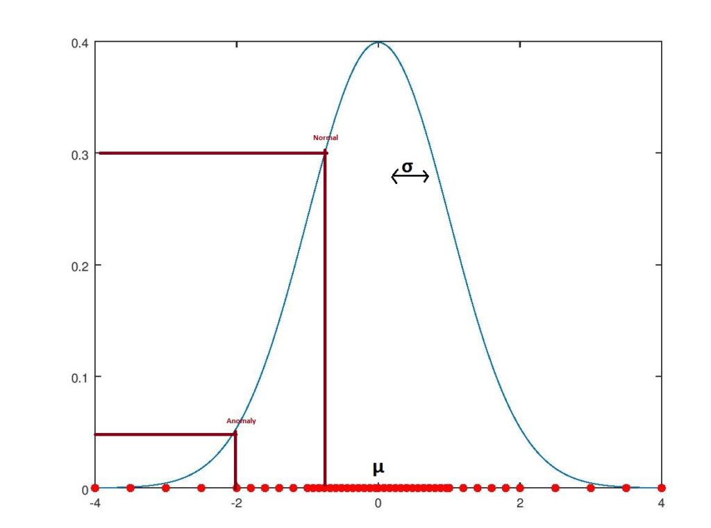
this section provides a brief description of how the gaussian function is used for anomaly detection. for a more detailed view, please refer to my previous post . the gaussian density function has a bell-shaped curve shape, as seen below:

regular data, which are the majority of the data, tend to be in the center of the bell-shaped curve, while anomalies on the edge are rarer. at the same time, we can see that points on the edge have lower function values (or probability, less than 0.1) compared to those in the center (close to 0.4).

following this example, we can say that every coming example that has a probability density function lower than 0.05 is an anomaly. of course, we can control the threshold value depending on our needs. big values mean that more anomalies are flagged and most of them are probably not anomalies. on the other hand, small values mean we may miss anomalies as the algorithm becomes more tolerant. there are several ways to calculate an optimal value, and one of the ways is described in my previous post .

the above example is one-dimensional, with data having only one feature. in reality, we have data with a lot more features and dimensions. to plot our data into the graph, we reduce the dimension of data using principal component analysis (pca) to two-dimensional (2d) or even three-dimensional (3d). here's an example with two dimensions:

notice how normal data tend to stay together in the middle of the first and second circles and anomalies are on the edges of the third circle. circles on the graph show how the gaussian bell curve is distributed among data (normally, it will be bell-shaped in 3d, but for simplicity, it is shown in 2d).

to place an example on a certain position in the bell-shaped graph, we need to calculate two components: µ (mean) and σ ₂ (variance).once we have calculated mean and variance, we can apply a fairly simple formula to get the density probability for new coming examples. if the probability is lower than a certain value ( sigma ), we flag it as an anomaly; otherwise, it is normal. find details about exploitation in my previous post .

spark and mllib

this section provides a brief description of both spark and mllib . for more detailed explanation and tutorial, check out the official website .

spark

apache spark is a cluster computing framework. spark help us execute jobs in parallel across different nodes in a cluster and then combine those results in one single result/response. it transforms our collection of data into a collection of elements distributed across nodes of the cluster called an rdd (resilient distributed dataset). for example, in a java program, we can transform a collection into an rdd capable of parallel operations like this:

javardd<labeledpoint> paralleledtestdata = sc.parallelize(collection);

parallel collections are cut into partitions and spark executes one task per partition, so we want to have two to four partitions per cpu. we can control the number of partitions spark created by defining another argument to the method with sc.parallelize(collection,partitionnumber) . besides collections coming from the application, spark is also capable of transforming data from the storage source supported by hadoop, including your local file system, hdfs, cassandra, hbase, and amazon s3.

after our data is transformed to an rdd, we can perform two kinds of parallel operations on cluster nodes. the transforming operation takes an rdd collection as input and returns a new rdd collection, like maps and actions, which take an rdd and return a single result like reduce, count, etc. regardless of the type, actions are lazy, similar to java 8 in the way that they do not run when defined but rather when requested . so, we can have an operation calculated several times when requested, and to avoid that, we can persist in memory or cache.

mllib

spark supports apis in java, scala, python, and r. it also supports a rich set of higher-level tools including spark sql for sql and structured data processing, mllib for machine learning, graphx for graph processing, and spark streaming.

mllib is spark’s machine learning (ml) library. it provided several ready-to-use ml tools like:

• ml algorithms
  • classification
  • regression
  • clustering
  • collaborative filtering
• featurization
  • feature extraction
  • transformation
  • dimensionality reduction
  • selection
• utilities
  • linear algebra
  • statistics
  • data handling

data preparation

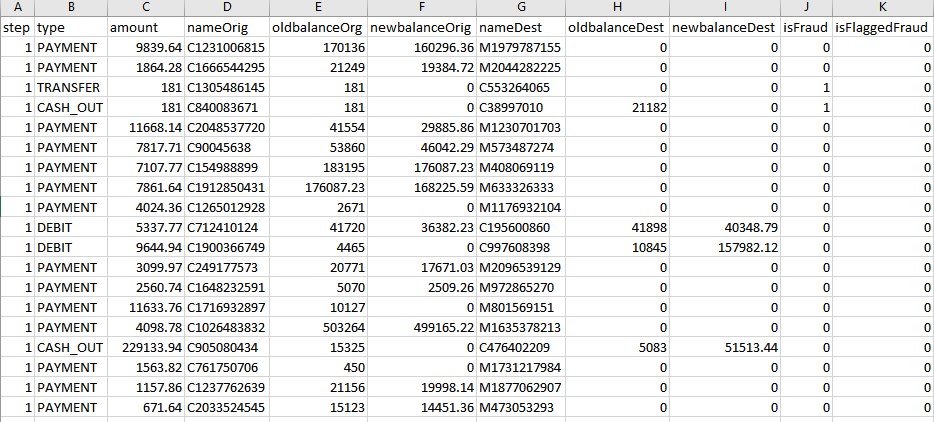
to get some insight on the data and how anomalies are distributed across regular data, see here . similar to the previous post , we need to prepare the data for the algorithm execution. here's what the data looks like:

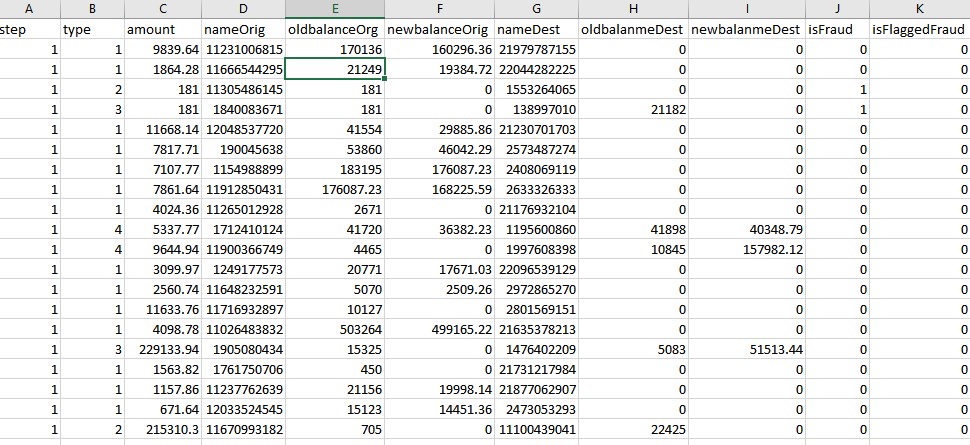
we need to convert everything into numbers. fortunately, most of the data are numbers — only nameorig and namedest start with a character like c , d , or m . we simply replace c with 1 , d with 2 , and m with 3 . also, we convert types from chars to numbers like below:

• payment = 1
• transfer = 2
• cash_out = 3
• debit = 4
• cash_in = 5

all the preparation is done with java code using the spark transformation operation map :

     file file = new file(algorithmconfiguration.getfilename());

        return sc.textfile(file.getpath()).
                map(line -> {
                    line = line.replace(transactiontype.payment.name(), "1")
                            .replace(transactiontype.transfer.name(), "2")
                            .replace(transactiontype.cash_out.name(), "3")
                            .replace(transactiontype.debit.name(), "4")
                            .replace(transactiontype.cash_in.name(), "5")
                            .replace("c", "1")
                            .replace("m", "2");
                    string[] split = line.split(",");
                    //skip header
                    if (split[0].equalsignorecase("step")) {
                        return null;
                    }
                    double[] featurevalues = stream.of(split)
                            .maptodouble(e -> double.parsedouble(e)).toarray();
                    if (algorithmconfiguration.ismakefeaturesmoregaussian()) {
                        frauddetectionalgorithmspark.this.makefeaturesmoregaussian(featurevalues);
                    }
                    //always skip 9 and 10 because they are labels fraud or not fraud
                    double label = featurevalues[9];
                    featurevalues = arrays.copyofrange(featurevalues, 0, 9);
                    return new labeledpoint(label, vectors.dense(featurevalues));
                }).cache();
    }
}

after that, the file should look like this:

because of the large file size and github file size limitation, data are not provided within the code. you can download the file from here , rename it alldata.csv (change constant file_name for the different name), and copy it into the folder data/ .

executing the algorithm

let's see step-by-step how we can execute the anomaly detection algorithm.

1. from all the data (seven million) we need to randomly choose a percentage for training, cross-validation, and test data . the code that will randomly pick up regular and fraudulent data for a dataset looks like this:

   collections.shuffle(regulardata);//randomly re order data
   collections.shuffle(anomalies);
   list<labeledpoint> regular = regulardata.stream().parallel().limit(normalsize).collect(tolist());
   list<labeledpoint> fraud = anomalies.stream().parallel().limit(fraudsize).collect(tolist());

   we run this code two times to get training and cross-validation data. what is left is the test data. we will see several percentage choices later on.
2. next, we will need µ (mean) and σ ₂ (variance) calculations, as they are crucial to getting the probability of new examples. the code looks like this:

   @override
   protected multivariatestatisticalsummary getmultivariatesummary(generateddata<javardd<labeledpoint>> traindata) {
       return statistics.colstats(traindata.regularandanomalydata.map(e -> e.features()).rdd());
   }

3. as mentioned earlier, once we have mean and variance using the gaussian formula, we can calculate the probability value. based on the probability value, we decide if it is an anomaly or a regular example. we compare the value with some threshold ( epsilon ); if it is lower, then we mark it as an anomaly, and if greater, we mark it as regular. choosing epsilon is crucial, as having small value can cause the algorithm to flag a lot of false fraud. on the other hand, with large values, we can miss fraud. we use cross-validation data with precision and recall to choose best epsilon.

   double bestepsilon = findbestepsilon(sc, crossdata, summary);
   resultssummary.setepsilon(bestepsilon);

4. now, we are ready to evaluate our algorithm on test data (we also do an optional evaluation on cross-validation data).

   testresult testresultfromtestdata = testalgorithmwithdata(sc, gettestdata(crossdata), summary, bestepsilon);
   filltestdataresults(resultssummary, testresultfromtestdata);
   
   testresult testresultfromcrossdata = testalgorithmwithdata(sc, crossdata.regularandanomalydata, summary, bestepsilon);
   fillcrossdataresults(resultssummary, testresultfromcrossdata);

before executing the algorithm, we need need to download data (it's not packed because of github's file size limitation), extract it, and copy and paste it as alldata.csv to the folder data/alldata.csv . the file location is configurable, as well as the file name. the algorithm can be tested with the data and various options through the configuration file at config/algorithm.properties , as shown below:

#60% of regular data used for training
traindatanormalpercentage=60

#0% of fraud data used for training
traindatafraudpercentage=0

#50% of frauds used as test data
testdatafraudpercentage=30
#20% of regular data used as test data
testdatanormalpercentage=20

#50% of frauds used as cross data
crossdatafraudpercentage=70
#20% of regular data used as cross data
crossdatanormalpercentage=20

#we can skip 11 features indexed from 0 to 10 ex 1,2,6,7
skipfeatures=1,2,3,6,7,8

#possible values :
#0->all
#1->payment
#2->transfer
#3->cash_out
#4->debit
#5->cash_in
transactiontypes=cash_out

#possible values spark and java_stream
runswith=spark

#how many times you want the algorithm to run
runstime=1

#make features more gaussian by powering current values
makefeaturesmoregaussian=true

filename=data/alldata.csv

hadoopapplicationpath=winutils-master/hadoop-2.8.1

after the configuration is changed, the application can be run on the java ide or in maven by running:

mvn clean install exec:java

depending on your machine and configuration, it may take some time (for me, it takes two minutes) for the application to finish. also, your computer may freeze a bit as, as spark gets the cpu to 100% at a certain point. also, expect a lot of memory to be used by the application (2-3 gb for me). you can see the result printed on the console or by looking at folder out/ ; there will a generated file *.txt with the output. as explained in my previous post , the algorithm is based on randomness, so you can configure it to run several times and expect one file per each execution.

experiments and results

from my experiments, i see that frauds are available only for two types: transfer and cash_out . transfer was investigated in details in my previous post . we achieved a pretty high rate: 99.7%.

when run only for the cash_out type and without skipping any columns/features, we get poor results:

resultssummary{
, run =0
, successpercentage=0.13532555879494654
, failpercentage=0.8646744412050534
trainregularsize=1340688
, trainfraudsize=0
, traintotaldatasize=0
, transactiontypes=[cash_out]
, timeinmilliseconds=58914
, testnotfoundfraudsize=1076
, testfoundfraudsize=180
, testflaggedasfraud=4873
, testfraudsize=1256
, testregularsize=446023
, testtotaldatasize=447279....

we are only able to find ~14% of frauds for this type. previously , we were able to improve a lot by making the feature more look like the gaussian bell curve, but unfortunately, that is not the case this time.

what we can do is look at our features and see if we can add or skip some features since features cam=n introduce confusion and noise rather than benefits. looking at the data source , we have following description of fraud, which can help:

" isfraud is the transactions made by the fraudulent agents inside the simulation. in this specific dataset, the fraudulent behavior of the agents aims to profit by taking control of customers' accounts and trying to empty the funds by transferring them to another account and then cashing out of the system."

it looks like fraud here is when a large amount or all of the funds are cashed out from the account. slowly, we start removing not-needed features; i found good results by removing features [1,2,3,7,8] or type ( amount , nameorig , oldbalancedest , newbalancedest ). when cashing out, the account from which the money is being taken is more important than the destination because the account may already have money and look pretty normal, but an empty source account may signal fraudulent behavior. we leave the destination account name, as it may help in case of fraudulent account names. the results look like :

finish within 70027
resultssummary{
, run =0
, successpercentage=0.8277453838678328
, failpercentage=0.17225461613216717
trainregularsize=1340058
, trainfraudsize=0
, traintotaldatasize=0
, transactiontypes=[cash_out]
, timeinmilliseconds=67386
, testnotfoundfraudsize=218
, testfoundfraudsize=1016
, testflaggedasfraud=139467
, testfraudsize=1234
, testregularsize=446808
, testtotaldatasize=448042

this is a huge improvement — we were able to go from14% to 82.77% by running all types together. also, it does not bring any better results with different skipped features (feel free to experiment, as not all of this is explored). i was able to get some results by skipping only amount (2), but this is still not satisfactory, as a lot of non-fraudulent activity was flagged(1,040,950).

finish within 128117
resultssummary{
, run =0
, successpercentage=0.8700840131498844
, failpercentage=0.12991598685011568
trainregularsize=3811452
, trainfraudsize=0
, traintotaldatasize=0
, transactiontypes=[all]
, timeinmilliseconds=125252
, testnotfoundfraudsize=325
, testfoundfraudsize=2153
, testflaggedasfraud=1040950
, testfraudsize=2478
, testregularsize=1272665
, testtotaldatasize=1275143

in this case, it's probably better to run the algorithm for each type. when a possible transaction is made, we run against its type. in this way, we will be able to detect fraudulent activity more appropriately, as transfer has a 99.7% rate and cash_out , 87% percent. still, for cash_out , we can say that the rate is not that satisfactory and maybe other approaches are worth try — but this has to be investigated first, and usually, intuition is wrong and costs a lot of time. since it's difficult to get more data in a finance application because of privacy, i would rather go in the direction of applying different algorithms here. when the data for cash_out were plotted, we got a view like below:

red = normal data,  magenta = not-found fraud, green = found frauds, and blue = wrongly flagged as fraud.

this graph shows that the problem is that the majority of fraud is contained in the center of the normal data and the algorithm struggles to detect them. still, i believe there could be other ways to mix features or even add more.

java stream vs. spark

we can configure the algorithm (see property runswith ) to run on spark or java 8 streams to manipulate the data. spark is a great framework if you want to run your code on several remote nodes on the cluster and aggregate results to a requested machine. in this post, the algorithm is executed locally and spark treats local resources like the number of cpu as target cluster resources. on the other hand, java 8 streams easily provides parallelism with collection.stram().parallel() (of course, on the running machine locally). so, as part of the experiment, java 8 streams were compared to spark on a single machine.

results show that java 8 streams are faster locally, even if not by much. java = 111,927 seconds and spark = 128,117 seconds — so basically, 16-25 seconds faster streams when it's run with all the data. please note that your computer results may differ; feel free to suggest new results.

since spark is optimized for distributed computing, it has some overhead with partitioning, tasks, and so on compared to java streams, which only need to think for the local machine and have the luxury to optimize a lot there. anyway, i can see the gap closing with the amount of data increasing even locally.

for a small amount of data, java 8 stream fits better, but for huge amounts of data, spark scales and fits better. maybe it's worth it to try spark configured on a cluster running maybe on aws rather than locally. for more details, please see the code for two java implementations handling the same exact algorithm but with nonessential small differences: frauddetectionalgorithmjavastream and frauddetectionalgorithmspark .