Exploring Zipf’s Law with Python, NLTK, SciPy, and Matplotlib
Join the DZone community and get the full member experience.
Join For Freezipf’s law states that the frequency of a word in a corpus of text is proportional to it’s rank – first noticed in the 1930′s. unlike a “law” in the sense of mathematics or physics, this is purely on observation, without strong explanation that i can find of the causes.
we can explore this concept fairly simply on a bit of text using nltk , which provides handy apis for accessing and processing text. there is a good textbook on the subject, “ natural language processing with python ” ( read my review ), with lots of motivating examples like this.
import nltk from nltk.corpus import reuters from nltk.corpus import wordnet reuters_words = [w.lower() for w in reuters.words()] words = set(reuters_words) counts = [(w, reuters_words.count(w)) for w in words] |
the first step of counting word frequencies takes quite a while (an hour or two). here are the top tokens (obviously not all words)
>>> [(w, c) for (w, c) in counts if c > 5000]
[('.', 94687), ('s', 15680), ('with', 6179), ("'", 11272),
('>', 7449), ('year', 7529), ('000', 10277), ('loss', 5124),
('u', 6392), ('pct', 9810), ('"', 6816), ('from', 8217),
('for', 13782), ('2', 6528), ('at', 7017), ('be', 6357),
('the', 69277), (';', 8762), ('he', 5215), ('net', 6989),
('is', 7668), ('it', 11104), ('in', 29253), ('billion', 5829),
('lt', 8696), ('-', 13705), ('of', 36779), ('&', 8698),
('to', 36400), ('vs', 14341), ('was', 5816), ('1', 9977),
 ('and', 25648), ('dlrs', 12417), ('by', 7101), ('its', 7402),
('mln', 18623), ('cts', 8361), ('on', 9244), ('that', 7540),
('3', 5091), ('a', 25103), (',', 72360), ('said', 25383),
('will', 5952)]
|
next, i joined this to wordnet data – while exploring zipf’s law, i want to test the hypthesis that common words are more likely to be irregular. we also generate the rankings of each word in the set, but frequencies, and by number of “synsets” in wordnet (synsets are sets meanings)
import scipy.stats as ss

amb = [(w, c, len(wordnet.synsets(w))) /
    for (w, c) in counts if len(wordnet.synsets(w)) > 0]

amb_p_rank = ss.rankdata([p for (w, c, p) in amb])
amb_c_rank = ss.rankdata([c for (w, c, p) in amb])

amb_ranked = zip(amb, amb_p_rank, amb_c_rank)

amb_ranked[100:110]
out[37]:
[('regulator', 2, 3, 8945.0, 5500.0),
 ('friend', 2, 5, 12344.0, 5500.0),
 ('feeling', 19, 19, 16810.0, 12979.0),
 ('sustaining', 7, 7, 14215.0, 10282.5),
 ('spectrum', 8, 2, 6142.0, 10684.5),
 ('consenting', 1, 2, 6142.0, 2218.5),
 ('resignations', 3, 3, 8945.0, 7215.5),
 ('dozen', 11, 2, 6142.0, 11554.0),
 ('affairs', 75, 5, 12344.0, 15397.5),
 ('mostly', 57, 2, 6142.0, 15038.0)]
|
the last line combines the data values together into one big list of tuples, for convenience. to do a quick test of zipf’s law, we can test that the rank correlates to the log of the count:
numpy.corrcoef(amb_c_rank, [math.log(c) for (w, c, p) in amb])
out[106]:
array([[ 1.        ,  0.95322962],
       [ 0.95322962,  1.        ]])
|
we can also demonstrate this a different way. first, we sort the records by occurence:
amb_ranked_sorted = sorted(amb_ranked, key=lambda (w, c, p, cr, pr): c) |
and then we take some samples. note how when we move by approximately 3x rank, the frequency goes down by about 1/3 (this will vary based on how the rank is counted, especially at the long tail where there are many matching counts in a row)
amb_ranked_sorted[-50]
out[121]: ('profit', 2960, 4, 10907.0, 17128.0)

amb_ranked_sorted[-150]
out[122]: ('major', 1000, 13, 16262.0, 17028.0)

amb_ranked_sorted[-450]
out[123]: ('goods', 408, 4, 10907.0, 16728.0)

amb_ranked_sorted[-1350]
out[124]: ('hope', 113, 9, 15215.0, 15827.5)
|
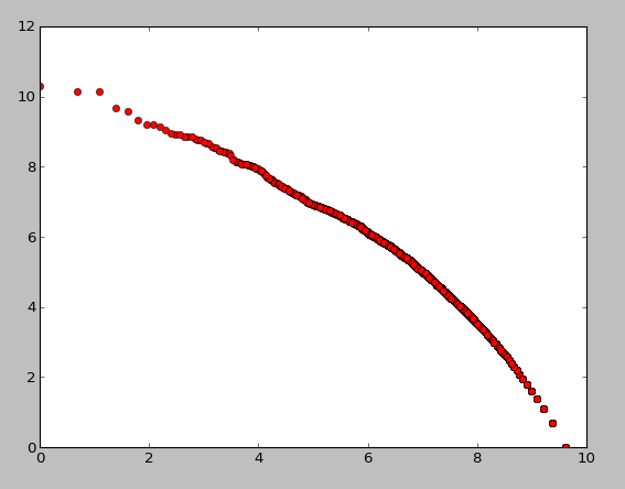
finally, we can plot this:
import matplotlib rev = [l-r+1 for r in amb_c_rank] plt.plot([math.log(c) for c in rev], [math.log(c) for (w, c, p) in amb], 'ro') |

this isn’t exactly straight, especially at the end, likely due to how ranks are computed, but it’s close. now we can plot the number of “meanings” in wordnet vs use in the reuters corpus:
plt.plot([c for (w,c,p) in amb], [p for (w,c,p) in amb], 'bs') out[150]: [<matplotlib.lines.line2d at 0x147ae950>] plt.show() |

the problem is that there is no notion of context, for instance the common word “at” is only referenced by the chemical element “astatine”:
wordnet.synsets('at')
out[149]: [synset('astatine.n.01'), synset('at.n.02')]
|
thus, a better technique is to look at verbs only.
def wordnet_verbs(w):
  synsets = wordnet.synsets(w)
  verbs = [w for w in synsets if w.pos == 'v']
  return verbs

amb_v = [(w, c, len(wordnet_verbs(w)), len(wordnet.synsets(w))) \
  for (w, c) in counts if len(wordnet_verbs(w)) > 0]

amb_v[100:110]
out[167]:
[('shoots', 1, 20, 22),
 ('suffice', 1, 1, 1),
 ('acquainting', 1, 3, 3),
 ('perfumes', 1, 2, 4),
 ('safeguard', 14, 2, 4),
 ('arrays', 4, 2, 6),
 ('crowns', 143, 4, 16),
 ('roll', 21, 18, 33),
 ('intend', 63, 4, 4),
 ('palms', 2, 1, 5)]

plt.plot([c for (w,c,vc,wc) in amb_v], [vc for (w,c,vc,wc) in amb_v], 'bs',\
         [c for (w,c,vc, wc) in amb_v], [wc for (w,c,vc,wc) in amb_v], 'ro')
|
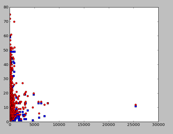
and, we can plot these (y axis is # of alternate meanings, x axis is frequency, blue is counts of verb meanings, and red is counts of word meanings).

there does seem to be a pattern here, but not what i expect – i would expect some straight-line upwards, with alternate meanings increasing with usage, which is actually the opposite. this likely means that the wordnet thesaurus counts are a poor indicator of irregularity. rather, words which have many meanings are discouraged in news writing, as they encourage ambiguity.
for a final note, lets look at what are these common words are:
[(w,c,vc,wc) for (w,c,vc,wc) in amb_v if vc > 40]
out[179]:
[('cut', 905, 41, 70),
 ('makes', 169, 49, 51),
 ('runs', 38, 41, 57),
 ('making', 369, 49, 52),
 ('gave', 208, 44, 44),
 ('breaks', 14, 59, 75),
 ('take', 745, 42, 44),
 ('broke', 40, 59, 60),
 ('run', 125, 41, 57),
 ('give', 303, 44, 45),
 ('cuts', 319, 41, 61),
 ('broken', 36, 59, 72),
 ('giving', 99, 44, 48),
 ('took', 140, 42, 42),
 ('breaking', 19, 59, 60),
 ('takes', 91, 42, 44),
 ('taken', 244, 42, 44),
 ('make', 592, 49, 51),
 ('taking', 197, 42, 44),
 ('given', 370, 44, 47),
 ('gives', 47, 44, 45),
 ('made', 987, 49, 52),
 ('break', 76, 59, 75),
 ('giveing', 1, 44, 44),
 ('cutting', 122, 41, 54),
 ('running', 73, 41, 52),
 ('ran', 29, 41, 41)]
|
“cut” has a staggering 70 entrieds in wordnet – many, but not all verbs. “has”, by contrast, has merely twenty.
Published at DZone with permission of Gary Sieling, DZone MVB. See the original article here.
Opinions expressed by DZone contributors are their own.

Comments