Application of Machine Learning Methods To Search for Rail Defects (Part 2)

To ensure traffic safety in railway transport, non-destructive inspection of rails is regularly carried out using various approaches and methods. One of the main approaches to determining the operational condition of railway rails is ultrasonic non-destructive testing [1]. Currently, the search for images of rail defects using the received flaw patterns is performed by a human. The successful development of algorithms for searching and classifying data makes it possible to propose the use of machine learning methods to identify rail defects and reduce the workload on humans by creating expert systems.

The complexity of creating such systems is described in [1, 3-6, 22] and is due, on the one hand, to the variety of graphic images obtained during multi-channel ultrasonic inspection of rails, and on the other hand, to the small number of data copies with defects (not balanced). One of the possible ways to create expert systems in this area is an approach based on the decomposition of the complex task of analyzing the entire multichannel defectogram into individual channels or their sets, characterizing individual types of defects. 

One of the most common rail defects is a radial bolt hole crack, referred to in the literature as “Star Crack” (Fig. 1). This type of defect is mainly detected by a flaw detector channel with a preferred central inclined angle of ultrasound input in the range of 38⁰- 45⁰ [1-2]. Despite the systematic introduction of continuous track on the railway network, the diagnosis of bolt holes is an important task [1-2], which was the reason for its identification and consideration in this work.

Figure 1 – Example of a radial crack in a rail bolt hole

• Purpose of the work: to compare the effectiveness of various machine learning models in solving the problem of classifying the states of bolt holes of railway rails during their ultrasonic examination.

The set purpose is achieved by solving the following problems:

• Data set generation and preparation
• Exploratory data analysis
• Selection of protocols and metrics for evaluating the operation of algorithms
• Selection and synthesis of implementations of classification models
• Evaluating the effectiveness of models on test data

Data Set Generation and Preparation

When a flaw detector equipped with piezoelectric transducers (PZT) travels along a railway track, ultrasonic pulses are emitted into the rail within a specified period. At the same time, receiving the PZT register reflected waves. The detection of defects by the ultrasonic method is based on the principle of reflecting waves from metal inhomogeneities, since cracks, including other inhomogeneities, differ in their acoustic resistance from the rest of the metal [1-5]. 

During ultrasonic scanning of rails, their structural elements and defects have acoustic responses, which are displayed on the defectogram in the form of characteristic graphic images (scans). Figure 2 shows examples of defectograms in the form of B-scan (“Bright-scan”) of sections of rails with a bolted connection, which were obtained by measuring systems of various types at an inclined angle of ultrasound input.

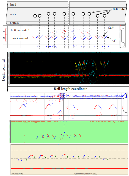
Figure 2 - Examples of individual flaw detection channels (B-scan) when scanning bolt holes of rails by flaw detectors of various companies

Individual scans of bolt holes (frames) can be separated from such flaw patterns, for example, by applying amplitude criteria (Fig. 3).

Figure 3 - Selection of frames with alarms of bolt holes from B-scan

Width W and length L of each frame are the same (Fig. 3), and are selected based on the maximum possible dimensions of bolt holes signaling and their flaws. Each such frame (instance) represents a part of the B-scan and therefore contains data on the coordinates, measurements, and sizes of each point, data from each of the two ultrasonic signal inputs on the rail (+/- 40⁰).  In work [3] such data frames are converted into a matrix with shape (60, 75), size 60 * 75 = 4500 elements in grayscale, classification network based on deep learning methods is built and successfully trained. However, the work does not consider alternative and less capacious options for data frame formats and does not show the capabilities of basic methods and machine learning models, so this work is intended to fill this drawback.

Various forms of radial cracks of rail bolt holes, their locations, and reflective properties of the surface lead to changing graphic images and, together with a defect-free state, generate a data set with the ability to distinguish 7 classes. In binary classification practice, it is common to assign class “1” to the rarer outcomes or conditions of interest, and class “0” to the common condition. In relation to the identification of defects, we will define a common and often encountered in practice defect-free state - class “0”, and defective states “1”-“6”. Each defect class is displayed on the flaw pattern as a characteristic image that is visible to experts during data decryption (Fig. 4). Although the presence or absence of a flaw (binary classification) is crucial during the operation of the railway track, we will consider the possibilities of classification algorithms and quantify which types of defects or flaws are more likely to be falsely classified as defect-free, which is a dangerous case in the diagnosis of rails.  Therefore, the classification problem is reduced in this work to an unambiguously multiclass classification.

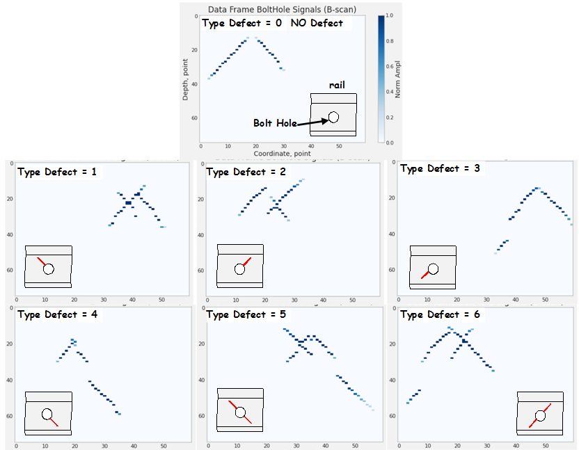
Figure 4 - Examples of B-scan frames (60, 75) with characteristic images of bolt holes with different radial cracks assigned to one of the 7 classes

Each instance of a class can be represented as a basic structure - rectangular data. To equalize the size of the instances, set the length of the table format to k = 60 records (30% more than the maximum possible), fill empty cells with zero values (Fig. 5a). Then the original instance can have the form (6, 60) or be reduced to the form of a flat array and described in 6*60=360 dimensional space (Fig. 5c), and on the B-scan graph it will look like Fig. 5b.

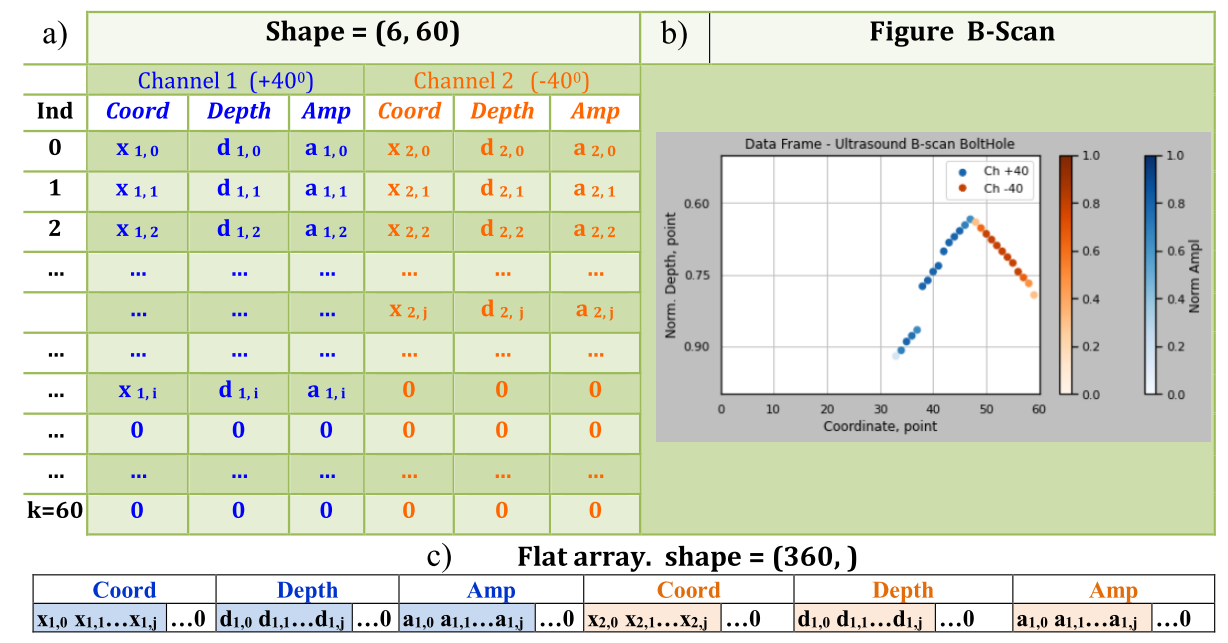
Figure 5 – Representation of a rectangular data instance

Selecting an Assessment Protocol

Collecting and annotating data from ultrasonic testing of rails is associated with significant difficulties, which are described in [3], so we will use a synthesized data set obtained using mathematical modeling. The essence of this approach is reflected in Fig. 6, and its applicability is shown in [3]. The term “synthesized data” is widely discussed when creating real-world visual objects, for example, on the nVIDEA blog [23]. This work extends the application of synthesized data into the field of non-destructive testing.

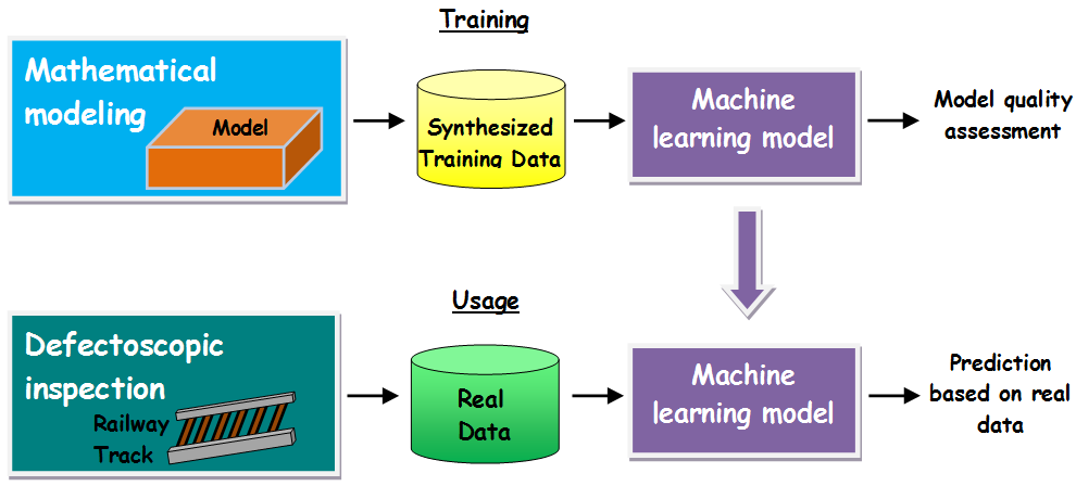
Figure 6 - Application of ML model

A sufficiently large number of data instances obtained on the basis of mathematical modeling allows us to avoid the problem of a rare class and choose a protocol for evaluating models in the form of separate balanced sets: training, verification, and testing. Let's limit the data sets: training data = 50,000, test data = 50,000, and validation data = 10,000 instances.

Choosing a Measure of Success

The absence of a difference in the relative sizes of classes (class balance) allows us to choose the accuracy indicator as a measure of success when training algorithms as a value equal to the ratio of the number of correctly classified instances to their total number. A single metric cannot evaluate all aspects of model applicability for a situation, so the model test step uses a confusion matrix, precision, and completeness measures for each class classifier.

Exploratory Data Analysis

Information about the balance of classes in the training, test, and validation set is presented in Fig. 7.

Figure 7 - Data Quantity Summary

The representation of the distribution of normalized alarm depths and their coordinates for the positive measuring channel Ch + 40⁰ and classes 0, 2, 3, and 6 is shown in Fig. 8. Distributions for Ch-40⁰ and channels 0, 1, 4, and 5 have a symmetrical pattern.

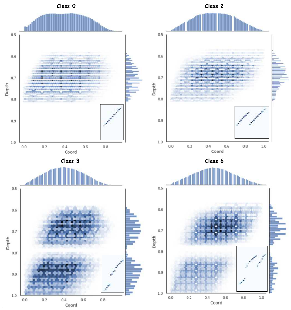
Figure. 8 – Distribution of normalized values of coordinates and depths of data from the Ch+400 measurement channel for classes 0, 2, 3, 6

The Principal Component Analysis (PCA) method was used as an Exploratory Data Analysis and determination of data redundancy, the two-dimensional representation of which can be represented in the form of Fig. 9. The central class is class 0, from which classes 2, 3, 6 and 1, 4, 5 are located on opposite sides, which corresponds to their graphical display on B-scan.

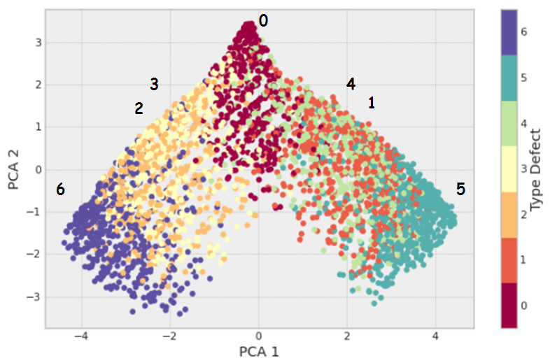
Figure 9 - Visualization of the two-dimensional representation of the PCA method

In general, a two-dimensional representation of classes has weak clustering, which indicates the need to use a higher dimension of data to classify them in the limit to the original flat size 6 * 60 = 360. The graph of the integral explainable variance as a function of the number of components of the PCA method (Figure 10a) shows that with 80 components, 98% of the variance is already explained, which indicates a high level of redundancy in the original data. This can be explained by the sparseness of the data, which shows the independence of the obtained 80 components of the PCA method from zero values (Fig. 10b).

Figure 10 – PCA: a) integral explained variance as a function of the number of components of the PCA method, b) contributions of predictive variables of a flat data array in projections on the PCA axes

Let's consider the assessment of the occupancy of data instances with non-zero values for each class (Fig. 11).

Fig. 11 - Assessment of occupancy with non-zero values of class instances

Note:

1. Similarity of ranges and quartiles of classes
2. Class 0 has the lowest median as the defect-free condition of the bolt hole is devoid of additional crack alarms.
3. Classes 5 and 6 have the highest median values, indicating high data filling due to the presence of alarms from the lower and upper radial crack of the bolt hole.
4. Classes 1-4 have similar median values, indicating that they are filled with data due to the presence of alarms only from the upper or lower radial crack of the bolt hole.
5. Classes 1 and 2, 3 and 4, 5 and 6, respectively, have similar medians and distributions, due to the symmetry of the data relative to the center of the bolt hole. 
6. The level of 80 components of the PCA method is lower than the median for classes 1-6, but is sufficient to describe 98% of the variances, which may indicate redundancy caused not only by zero values in the data. A possible explanation could be the fact that the amplitude values of the alarms do not change much in each class and have a weak effect on the variance. This fact is confirmed by the practice of searching for defects, in which flaw detectors do not often use the amplitude parameter.

To assess the complexity of the upcoming Exploratory Data Analysis task, the multidimensional structure of the input data was studied using Manifold learning techniques (Manifold learning): 

• Random projection embedding
• Isometric Mapping (Isomap)
• Standard Locally linear embedding (LLE)
• Modified Locally linear embedding (LLE)
• Local Tangent Space Alignment embedding (LTSA)
• Multidimensional scaling (MDS)
• Spectral embedding
• t-distributed Stochastic Neighbor Embedding (t-SNE)

Also, techniques that can be used for controlled dimensionality reduction and allowing data to be projected into a lower dimension:

• Truncated SVD embedding
• Random Trees embedding
• Neighborhood Components Analysis (NCA)
• Linear Discriminant Analysis (LDA)

The results of the algorithms for embedding data from 3,000 samples of the original shape (6, 60) into two-dimensional space are presented in Fig. 12.

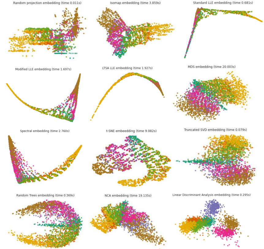
Figure 12 – Embedding data into two-dimensional space using various techniques (the color of the dots represents the class)

For Manifold learning methods, the data in the graphs is poorly spaced in parametric space, which characterizes the predictable complexity of data classification by simple supervised algorithms. 

Note also that the method of controlled dimensionality reduction Linear Discriminant Analysis shows good data grouping and can be a candidate for a classification model.

Development of Data Classification Models

Basic Model

The prediction accuracy of each class out of seven possible with a random classifier is 1 / 7 = 0.143 and is the starting point for assessing the statistical power (quality) of future models. 

As a base model, we will choose Gaussian Naive Bayes, which is often used in such cases.  A code fragment for fitting a model on training data and its prediction on test data:

from sklearn.naive_bayes import GaussianNB
from sklearn.metrics import accuracy_score
from sklearn.metrics import confusion_matrix
batch = 50000
train_gen = Gen_2D_Orig_Arr(train_dir, batch_size=batch, num_classes=7)
Xtrain, ytrain = next(train_gen) #  Xtrain.shape = (50 000, 6, 60, 1),  
                                 #  ytrain.shape = (50 000, 7)
Xtrain = np.reshape(Xtrain, (batch, Xtrain.shape[1] * Xtrain.shape[2])) # Xtrain.shape = (50 000, 360)
ytrain = np.argmax(ytrain, axis=1)  # ytrain.shape = (50 000,)

test_gen = Gen_2D_Orig_Arr(test_dir, batch_size=batch, num_classes=7)
Xtest, ytest = next(test_gen)
Xtest = np.reshape(Xtest, (batch, Xtest.shape[1] * Xtest.shape[2]))
ytest = np.argmax(ytest, axis=1)  # ytest.shape = (50 000,)
model = GaussianNB()
model.fit(Xtrain, ytrain)
start_time = time()
y_model =  model.predict(Xtest) # y_model.shape = (50 000,)
timing = time() - start_time
acc = accuracy_score(ytest, y_model)
print('acc = ', acc)
print(classification_report(ytest, y_model, digits=4))
mat = confusion_matrix(ytest, y_model) # mat.shape = (7, 7)
fig =  plt.figure(figsize=(10, 6), facecolor='1')
ax = plt.axes()
sns.heatmap(mat, square=True, annot=True, cbar=False, fmt="d", linewidths=0.5)
plt.xlabel('сlass qualifiers')
plt.ylabel('true value');
print(f'{timing:.3f} s -  Predict time GaussianNB')

The resulting difference matrix and summary report on model quality are presented in Fig. 13 a and b. The trained model has statistical power, as it has an overall accuracy of 0.5819, which is 4 times higher than the accuracy of a random classifier. Despite the rather low accuracy of the model, we will consider the specific relationship between the qualitative indicators of its work and the graphical representation of the projected data using the Linear Discriminant Analysis method (Fig. 13c). 

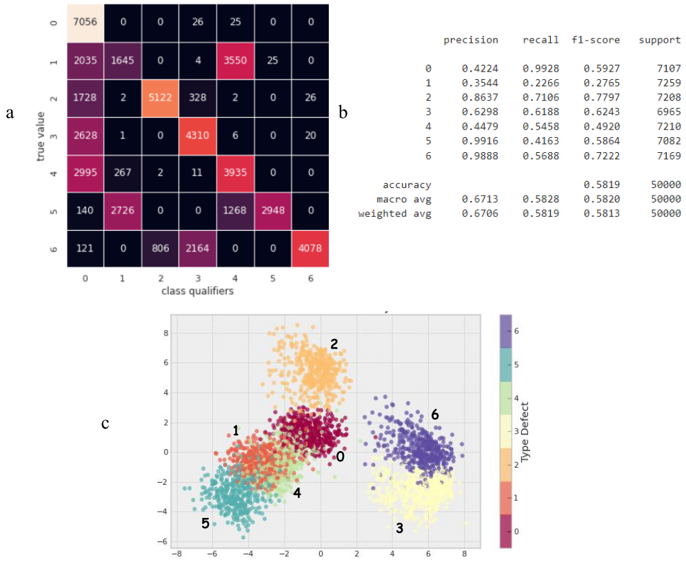
Figure 13 - Summary Quality Assessments of the Gaussian Naïve Bayesian Model: a) dissimilarity matrix showing model misclassification rates; b) a report on the qualitative indicators of the model’s performance in the form of various accuracy metrics; c) projection of data into two-dimensional space using the Linear Discriminant Analysis method

The projected data of class 6 are the most distant from most points of other classes (Fig. 13c), which is reflected in the high precision of its classifier equal to 0.9888, however, the closeness of the representation of class 3 reduced the recall of classifier 6 to 0.5688 due to false negative predictions, which are expressed by the error rate equal to 2164 in the dissimilarity matrix. 

The projection of class 5 is also removed, which is reflected in the high precision of its classifier equal to 0.9916, however, it has intersections with classes 1 and 4, which affected the completeness of the classifier equal to 0.4163, due to erroneous predictions with frequencies of 2726 and 1268 for classifiers 1 and 4, respectively.

The projection of class 1 has intersections with classes 5, 4, and 0, while, accordingly, classifier 1 has false positives with a frequency of 2726 for class 5 and false negatives with frequencies of 2035 and 3550 in favor of classifiers 0 and 4. 

Similar relationships are observed for other classes. One of the interesting ones is the behavior of classifier 0. Defect-free class 0 is in the middle of the projections, which corresponds to its graphic image, which is closest to classes 1, 2, 3, and 4 and most distinguishable from classes 5 and 6 (Fig. 4). Classifier 0 recognizes its data class well, which causes the highest recall score of 0.9928, but has numerous false positives in classes 1, 2, 3, 4 with a precision of 0.4224, that is, classes with defects are often classified as a defect-free class (class 0 ), which makes the Gaussian Naive Bayes model completely unsuitable for flaw detection purposes. The resulting Gaussian Naive Bayes classifier is simple enough to describe complex data structure.

Linear Discriminant Analysis (LDA) Classifier Model

Preliminary analysis based on data dimensionality reduction showed a good grouping of classes within the Linear Discriminant Analysis method (Fig. 12), which served as a motivation for its use as one of the next models:

from sklearn.discriminant_analysis import LinearDiscriminantAnalysis
lda_model = LinearDiscriminantAnalysis(solver='svd', store_covariance=True)
lda_model.fit(Xtrain, ytrain)
y_model = lda_model.predict(Xtest)
acc = accuracy_score(ytest, y_model)
print(classification_report(ytest, y_model, digits=4))
mat = confusion_matrix(ytest, y_model)
fig = plt.figure(figsize=(10, 5), facecolor='1')
sns.heatmap(mat, square=True, annot=True, cbar=False, fmt='d', linewidths=0.5)
plt.xlabel('сlass qualifiers')
plt.ylabel('true value');

The results of its training and prediction are presented in Fig. 14. The overall accuracy of the model was 0.9162, which is 1.57 times better than the accuracy of the basic model. However, classifier 0 has a large number of false positives for classes 2 and 4 and its precision is only 0.8027, which is also not a satisfactory indicator for the purposes of its practical application.

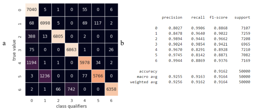
Figure 14 – Summary assessments of the quality of work of the Linear Discriminant Analysis (LDA) classifier 

The hypothesis about the possible lack of training data set to increase the accuracy of the LDA model is not confirmed, since the constructed “learning curve” presented in Fig. 15 shows a high convergence of the training and testing accuracy dependencies at the level of 0.92 with a training set size of 5000 – 6000 items:

from sklearn.model_selection import learning_curve
gen = Gen_2D_Orig_Arr(train_dir, batch_size=8000,  num_classes=7)
x1, y1 = next(gen) #  x1.shape = (8000, 6, 60, 1),  y1.shape = (8000, 7)
x1 = np.reshape(x1, (batch, x1.shape[1] * x1.shape[2])) # x1.shape = (8000, 360)
y1 = np.argmax(y1, axis=1)  # y1.shape = (8000,)
N,  train_sc, val_sc = learning_curve(lda_model, x1, y1, cv=10,  
   train_sizes=np.linspace(0.04, 1, 20))
rmse_tr = (np.std(train_sc, axis=1))
rmse_vl = (np.std(train_sc, axis=1))

fig, ax = plt.subplots(figsize=(10, 6))
ax.plot(N, np.mean(train_sc, 1), '-b', marker='o', label='training')
ax.plot(N, np.mean(val_sc, 1),   '-r', marker='o', label='validation')
ax.hlines(np.mean([train_sc[-1], val_sc[-1]]), 0, 
    N[-1], color='gray', linestyle='dashed')
ax.fill_between(N, np.mean(train_sc, 1) –
    3 * rmse_tr, np.mean(train_sc, 1) + 
    3 * rmse_tr, color='blue', alpha=0.2)
ax.fill_between(N, np.mean(val_sc, 1) –
                3 * rmse_vl, np.mean(val_sc, 1)+ 
                3 * rmse_vl, color='red',  alpha=0.2)
ax.legend(loc='best');
ax.set_xlabel('training size')
ax.set_ylabel('score')
ax.set_xlim(0, 6500)
ax.set_ylim(0.7, 1.02);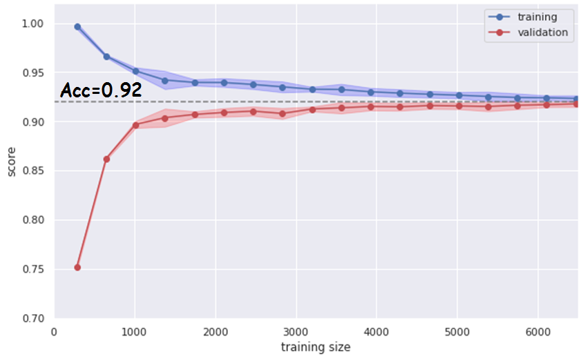

Figure 15: High convergence of the training and testing accuracy dependencies at the level of 0.92 with a training set size of 5000 – 6000 items

When trying to create such a classification system, manufacturers of flaw detection equipment are faced with the difficulty of assessing the dependence of the predictive accuracy of the system on the number of items in the data set that need to be obtained in the process of rail diagnostics. The resulting learning curve based on model data allows in this case to estimate this number in the range of 5,000 – 6,000 copies, to achieve an accuracy of 0.92 within the framework of the LDA algorithm.

The decreasing dependence of the learning curve on the training data (blue color in Fig. 15) of the LDA classifier shows that it is simple enough for a complex data structure and there is a justified need to find a more complex model to improve prediction accuracy.

Dense Network

One of the options for increasing forecast accuracy is the use of fully connected networks. The option of such a structure with the found optimal parameters using the tool Keras_tuner shown in Figure 16a, the accuracy of the model increased compared to the previous method to 0.974 (Figure 16b), and the precision of the zero class classifier to 0.912.

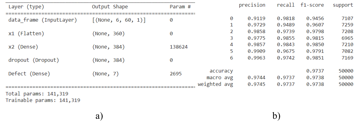
Fig. 16 – Model structure and accuracy indicators

The progressive movement to increase the accuracy of the prediction due to the use of more complex (computationally costly) machine learning algorithms shows the justifiability of actions to create increasingly complex models.

Support Vector Machine (SVM)

The use of a support vector algorithm with a core as a radial basis function and over-the-grid model hyperparameters using the GridSearchCV class from the scikitlearn machine learning library made it possible to obtain a model with improved quality parameters Fig. 17.

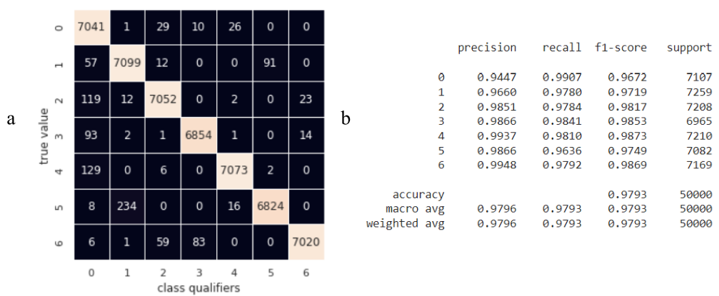
Fig. 17 - Summary of Classifier Performance Estimates Based on Support Vector Method (SVM)

The use of the SVM method increased both the overall prediction accuracy to 0.9793 and the precision of the null classifier to 0.9447. However, the average running time of the algorithm on a test data set of 50,000 instances with the initial dimension of each 360 was 9.2 s and is the maximum for the considered classifiers. Reducing the model's operating time through the use of pipelines in the form of techniques for reducing the dimensionality of the source data and the SVM algorithm did not allow for maintaining the achieved accuracy.

Random Forest Classifier

The RandomForestClassifier classifier based on an ensemble of random trees implemented in the scikitlearn package is one of the candidates for increasing the classification accuracy of the data under consideration:

from sklearn.ensemble import RandomForestClassifier
rf = RandomForestClassifier(n_estimators=50)

The performance estimates of the random forest algorithm of 50 trees on the test set are shown in Fig. 18. The algorithm made it possible to increase both the overall prediction accuracy to 0.9991 and an important indicator in the form of precision of the null classifier to 0.9968. The zero class classifier makes the most mistakes in classes 1-4 that are similar in graphical representation. The precision of classifiers of classes 1-4 is high and is reduced due to errors in favor of classes 5 and 6, which is not critical in identifying flaws.

The average running time of the algorithm according to the prediction of the test data set on the CPU was 0.7 s, which is 13 times less than the running time of SVM with an increase in accuracy of 0.02%.

Fig. 18 – Summary assessments of the quality of the classifier based on the random trees method

The learning curve of the RandomForestClassifier classifier is presented in Fig. 19 shows a high level of optimality of the constructed model:

• With increasing training data, the efficiency of the model does not decrease, which indicates the absence of the undertraining effect.
• The efficiency assessment at the training and testing stage converges and has high values with a difference of no more than 0.028, which may indicate that the model is not overtrained.

Fig. 19 – Learning curve of the RandomForestClassifier

The resulting learning curve allows us to estimate the minimum required number of samples of each class to achieve acceptable accuracy at the level of 0.98: 1550 data copies, that is, 1550 / 7 = 220 samples for each of the 7 classes.

The high accuracy and speed of the random forest algorithm allow you to assess the magnitude of the influence (importance) of all 360 predictive variables on the overall accuracy of the model. The evaluation was carried out by obtaining the average decreasing accuracy of the model by randomly mixing one of the variables, which had the effect of removing its predictive power. Fig. 20 shows the result of a code fragment for assessing the importance of variables on the accuracy of the model:

rf = RandomForestClassifier(n_estimators=10)
gen = Gen_2D_Orig_Arr(train_dir, batch_size=8000)
x1, y1 = next(gen) #  x1.shape = (8000, 6, 60, 1),  y1.shape = (8000, 7)
x1 = np.reshape(x1, (batch, x1.shape[1] * x1.shape[2]))  # x1.shape = (8000, 360)
y1 = np.argmax(y1, axis=1)  # y1.shape = (8000,)
Xtrain, Xtest, ytrain, ytest  = train_test_split(x1, y1, test_size=0.5)
rf.fit(Xtrain, ytrain)
acc = accuracy_score(ytest, rf.predict(Xtest)) 
print(acc)
scores = np.array([], dtype=float)
for _ in range(50):
  train_X, valid_X, train_y, valid_y = train_test_split(x1, y1, test_size=0.5)
  rf.fit(train_X, train_y) 
  acc = accuracy_score(valid_y, rf.predict(valid_X)) 
  for column in range(x1.shape[1]):
    X_t = valid_X.copy()
    X_t[:, column] = np.random.permutation(X_t[:, column])
    shuff_acc = accuracy_score(valid_y, rf.predict(X_t))
    scores = np.append(scores, ((acc  - shuff_acc) / acc))
scores = np.reshape(scores, (50, 360)) 
sc = scores.mean(axis=0)
fig, ax = plt.subplots(figsize=(10, 4))
ax.plot(sc, '.-r')
ax.set_xlabel('Predictive variables')
ax.set_ylabel('Importance')
ax.set_xlim([0, 360])
ax.xaxis.set_major_locator(plt.MaxNLocator(6))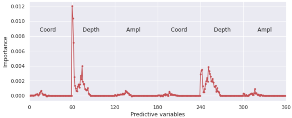

Figure 20 - Assessment of the importance of predictive variables by RandomForestClassifier-based model accuracy

The graph in Fig. 20 shows that the most important predictive variables are from 60 to 85 for channel +40 and from 240 to 265 for channel -40, which determine the depth of the alarm. The presence of peaks at the beginning and end of each range indicates even greater predictive importance of the depths of the beginning and end of alarms. The total number of important variables can be estimated at 50.

The importance of variables determining the coordinates and amplitude of the alarm in each data instance is much lower. This assessment is consistent with the assumptions made during the exploration analysis. Training RandomForestClassifier on the entire training data set without amplitudes showed an overall accuracy of 0.9990, without amplitudes and coordinates - 0.9993. Excluding from consideration such parameters as amplitude and coordinate for each data instance reduces the size of the data under consideration to (2, 60) = 120 predictive variables without reducing accuracy. The obtained result allows us to use only the alarm depth parameter for the purpose of data classification.

The accuracy achieved by RandomForestClassifier is sufficient and solves the problem of classifying defects in bolt holes. However, for the purpose of generalizing the capabilities, let’s consider a class of deep learning models based on a convolutional neural network.

Deep Learning (DL) Model

Synthesis and training of a convolutional network requires an iterative process with the search for the best structures and optimization of their hyperparameters. Fig. 21 shows the final version of a simple network structure in the form of a linear stack of layers and the process of its training.

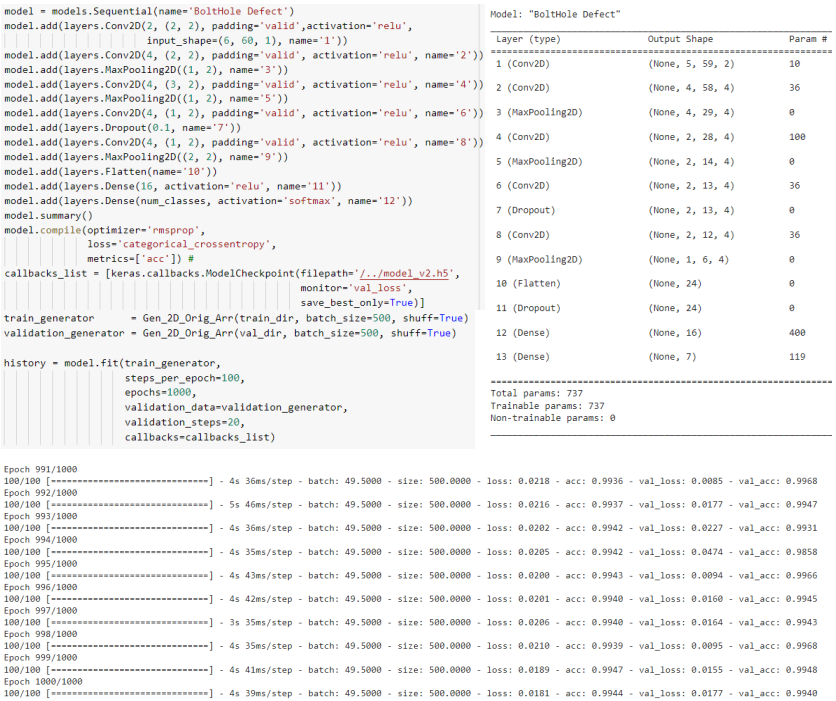
Figure 21 – Model structure and report on its training process

The results of training and forecasting of the convolutional neural network are presented in Fig. 21. The overall accuracy of the model on test data was 0.9985, which is 1.71 times better than the accuracy of the base model. The number of false positives of classifier 0 is 2+24+6+2=34 out of all 42893 defective instances (Fig. 22a). The average time for predicting test data on the CPU was 4.55 s.

Figure 22 – Summary assessments of the quality of work of a trained network based on CNN on test data

One of the important tasks of the resulting classifier in its practical use will be the accurate determination of the defect-free class (class 0), which will eliminate the false classification of defective samples as non-defective. It is possible to reduce the number of false positives for a defect-free class by changing the probability threshold. To estimate the applicable threshold cut-off level, a binarization of the multi-class problem was carried out with the selection of a defect-free state and all defective states, which corresponds to the “One vs Rest” strategy. By default, the threshold value for binary classification is set to 0.5 (50%). With this approach, the binary classifier has the quality indicators shown in Fig. 23.

Fig. 23 – Qualitative indicators of a binary classifier at a cutoff threshold of 0.5

The resulting precision for the “No defect” class was 0.9952, the same as for the multiclass classifier for class “0”. The use of the sklearn.metrics.precision_recall_curve function allows you to reflect changes in the precision and completeness of a binary classifier depending on a changing cutoff threshold (Fig. 24a). At a cutoff threshold of 0.5, the value of false positives is 34 samples (Fig. 24b). The maximum level of precision and completeness of the classifier is achieved at the point of intersection of their graphs, which corresponds to a cutoff threshold of 0.66. At this point, the classifier reduces the number of false positives for the “No defect” class to level 27 (Fig. 24b). Increasing the threshold to the level of 0.94 allows you to reduce false positives to a value of 8, due to an increase in false negatives to 155 samples (Fig. 24b) (decreasing the completeness of the classifier). A further increase in the cutoff threshold significantly reduces the completeness of the classifier to an unacceptable level (Fig. 24a).

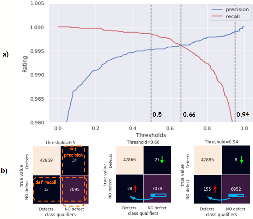
Figure 24 – Effect of the cut-off threshold: a) graph of changes in precision and completeness depending on the change in the cut-off threshold value (precision-recall curve); b) dissimilarity matrices at different cutoff thresholds

With a set cutoff threshold of 0.94, the qualitative assessments of the classifier are shown in Fig. 25. Precision for the “No defect” class increased to 0.9989.

Fig. 25 – Qualitative indicators of a binary classifier with a cutoff threshold of 0.94

Eight false-positive classified data samples with characteristic graphical signs of defects highlighted are shown in Fig. 26.

Fig. 26 - Eight false-positive classified samples

Of the above graphic images, the controversial ones are the samples marked “controversial”, which indicate the presence of a very short radial crack, which is difficult to classify as a defect. The remaining 6 samples are the classifier error. Note the qualitative indicator in the form of the absence of false classification of samples with defects in the form of a significant length of the radial crack. Such samples are most easily classified during manual analysis by flaw detectors.

Further increase in model accuracy is possible through the use of ensembles of the resulting models: DL and RandomForestClassifier. The considered models can be added to the ensemble, but obtained with a different input data format, including the direct Bscan format, as shown in [3]. 

Conclusions and Discussion

The main quality indicators of the developed models for classifying defects in bolt holes are summarized in the diagram in Fig. 27. The gradual and reasonable complication of classification models is reflected in the diagram in the form of an increase in both the overall accuracy of the models (blue color) and an important indicator in the form of class 0 precision (orange color). Maximum accuracy rates above 0.99 were achieved by models based on random forest and convolutional neural networks. At the same time, the random forest model has the advantage of less time spent on prediction.

Fig. 27 – Highlighted quality indicators of the considered classification models

 In This Work

1. The possibility of searching for defects on an ultrasonic flaw detector is shown by decomposing it into separate channels with data and allocating individual diagnostic sites.
2. An assessment is made of the influence of predictive variables in the form of amplitude and coordinates on the quality of classification.
3. An estimate is given of the required amount of data set to build a classification model of defects in bolt holes with an accuracy of 98%, which can serve as a guide for manufacturers of flaw detection equipment when creating automatic expert systems.
4. The possibility of achieving high accuracy rates for classifying the states of rail bolt holes based on classical machine learning algorithms is shown.
5. Qualitative assessments of the operation of the deep learning model are obtained and show the possibility and feasibility of using a convolutional neural network architecture for the synthesis of segmentation networks for searching for defects in continuous flaw patterns (B-scan).

References

• [1] Markov AA, Kuznetsova EA. Rail flaw detection. Formation and analysis of signals. Book 2. Decoding of defectograms. Saint Petersburg: Ultra Print; 2014. 
• [2] Markov AA, Mosyagin VV, Shilov MN, Fedorenko DV. AVICON-11: New Flaw-Detector for One Hundred Percent Inspection of Rails. NDT World Review. 2006; 2 (32): 75-78. Available from: http://www.radioavionica.ru/activities/sistemy-nerazrushayushchego-kontrolya/articles/files/razrab/33.zip [Accessed 14th March 2023].
• [3] Kaliuzhnyi A. Application of  Model Data for Training the Classifier of Defects in Rail Bolt Holes in Ultrasonic Diagnostics. Artificial Intelligence Evolution [Internet]. 2023 Apr. 14 [cited 2023 Jul. 28];4(1):55-69. DOI: https://doi.org/10.37256/aie.4120232339
• [4] Kuzmin EV, Gorbunov OE, Plotnikov PO, Tyukin VA, Bashkin VA. Application of  Neural Networks for Recognizing Rail Structural Elements in Magnetic and Eddy Current Defectograms. Modeling and Analysis of Information Systems. 2018; 25(6): 667-679. Available from: doi:10.18255/1818-1015-2018-6-667-679
• [5] Bettayeb F, Benbartaoui H,  Raouraou B. The reliability of the ultrasonic characterization of welds by the artificial neural network. 17th World Conference on Nondestructive Testing; 2008;  Shanghai, China. [Accessed 14th March 2023]
• [6] Young-Jin C, Wooram C, Oral B.  Deep Learning-Based Crack Damage Detection Using Convolutional Neural Networks.  Computer-Aided Civil and Infrastructure Engineering.   2017; 32(5): 361-378. Available from: doi: 10.1111/mice.12263
• [7] Heckel T, Kreutzbruck M, Rühe S, High-Speed Non-Destructive Rail Testing with Advanced Ultrasound and Eddy-Current Testing Techniques.  5th International workshop of   NDT experts - NDT in progress 2009 (Proceeding).  2009; 5: 101-109. [Accessed 14th March 2023].
• [8] Papaelias M, Kerkyras S, Papaelias F, Graham K. The future of rail inspection technology and the INTERAIL FP7 project.  51st Annual Conference of the British Institute of   Non-Destructive Testing 2012, NDT 2012. 2012 [Accessed 14th March 2023].
• [9]  Rizzo P, Coccia S, Bartoli I, Fateh M.  Non-contact ultrasonic inspection of rails and signal processing for automatic defect detection and classification.  Insight. 2005; 47 (6): 346-353. Available from:  doi: 10.1784/insi.47.6.346.66449
• [10] Nakhaee MC, Hiemstra D, Stoelinga M, van Noort M. The Recent Applications of Machine Learning in Rail Track Maintenance: A Survey. In: Collart-Dutilleul S, Lecomte T, Romanovsky A. (eds.) Reliability, Safety, and Security of Railway Systems. Modelling, Analysis, Verification, and Certification. RSSRail 2019. Lecture Notes in Computer Science(), vol 11495. Springer, Cham; 2019.pp.91-105. Available from:  doi: 10.1007/978-3-030-18744-6_6.
•  [11] Jiaxing Y, Shunya I, Nobuyuki T. Computerized Ultrasonic Imaging Inspection: From Shallow to Deep Learning. Sensors. 2018; 18(11): 3820. Available from:   doi:10.3390/s18113820
• [12] Jiaxing Y, Nobuyuki T. Benchmarking Deep Learning Models for Automatic Ultrasonic Imaging Inspection. IEEE Access. 2021; 9: pp 36986-36994. Available from:    doi:10.1109/ACCESS.2021.3062860
• [13] Cantero-Chinchilla S,  Wilcox PD, Croxford AJ. Deep learning in automated ultrasonic NDE - developments, axioms, and opportunities. Eprint arXiv:2112.06650. 2021. Available from:  doi: 10.48550/arXiv.2112.06650
• [14] Cantero-Chinchilla S,  Wilcox PD, Croxford AJ. A deep learning-based methodology for artifact identification and suppression with application to ultrasonic images. NDT & E International. 202; 126,  102575. Available from: doi: 10.1016/j.ndteint.2021.102575 
• [15] Chapon A, Pereira D, Toewsb M, Belanger P. Deconvolution of ultrasonic signals using a convolutional neural network. Ultrasonics. Volume 111, 2021; 106312. Available from: doi: 10.1016/j.ultras.2020.106312
• [16] Medak D, Posilović L, Subasic M, Budimir M. Automated Defect Detection From Ultrasonic Images Using Deep Learning. IEEE Transactions on Ultrasonics, Ferroelectrics, and Frequency Control. 2021; 68(10): 3126 – 3134. Available from: doi: 10.1109/TUFFC.2021.3081750 
• [17] Virkkunen I, Koskinen T. Augmented Ultrasonic Data for Machine Learning.  Journal of   Nondestructive Evaluation. 2021; 40: 4. Available from: doi:10.1007/s10921-020-00739-5
• [18] Veiga JLBC, Carvalho AA, Silva IC. The use of artificial neural network in the classification of pulse-echo and TOFD ultra-sonic signals. Journal of the Brazilian Society of Mechanical Sciences and Engineering. 2005; 27(4): 394-398 Available from: doi:10.1590/S1678-58782005000400007
• [19] Posilovića L, Medaka D, Subašića M, Budimirb M, Lončarića S. Generative adversarial network with object detector discriminator for enhanced defect detection on ultrasonic B-scans. Eprint arXiv:2106.04281v1 [eess.IV]. 2021. Available from: https://arxiv.org/pdf/2106.04281.pdf
• [20] Markov AA, Mosyagin VV, Keskinov MV. A program for 3D simulation of signals for ultrasonic testing of specimens.  Russian Journal of Nondestructive Testing. 2005; 41: 778-789. Available from: doi: 10.1007/s11181-006-0034-3
• [21]  Shilov M.N., Methodical, algorithmic, and software for registration and analysis of defectograms during ultrasonic testing of rails [dissertation]. [Saint-Petersburg]: Saint-Petersburg State University of Aerospace Instrumentation; 2007. p 153. 
• [22] A. Kaliuzhnyi. Using Machine Learning To Detect Railway Defects. 
• [23] NVIDIA Blog