Understanding Bayesian Modeling and Probabilistic Programming for Machine Learning

Traditional machine learning (ML) models and AI techniques often suffer from a critical flaw: they lack uncertainty quantification. These models typically provide point estimates without accounting for the uncertainty surrounding their predictions. This limitation undermines the ability to assess the reliability of the model's output. Moreover, traditional ML models are data-hungry and often require correctly labeled data, and as a result, tend to struggle with problems where data is limited. Furthermore, these models lack a systematic framework for incorporating expert domain knowledge or prior beliefs into the model. Without the ability to leverage domain-specific insights, the model might overlook crucial nuances in data and tend not to perform up to its potential. ML models are becoming more complex and opaque, while there is a growing demand for more transparency and accountability in decisions derived from data and AI. 

Probabilistic Programming: A Solution To Addressing These Challenges

Probabilistic programming provides a modeling framework that addresses these challenges. At its core lies Bayesian statistics, a departure from the frequentist interpretation of statistics. 

Bayesian Statistics

In frequentist statistics, probability is interpreted as the long-run relative frequency of an event. Data is considered random and a result of sampling from a fixed-defined distribution. Hence, noise in measurement is associated with the sampling variations. Frequentists believe that probability exists and is fixed, and infinite experiments converge to that fixed value. Frequentist methods do not assign probability distributions to parameters, and their interpretation of uncertainty is rooted in the long-run frequency properties of estimators rather than explicit probabilistic statements about parameter values.

In Bayesian statistics, probability is interpreted as a measure of uncertainty in a particular belief. Data is considered fixed, while the unknown parameters of the system are regarded as random variables and are modeled using probability distributions. Bayesian methods capture uncertainty within the parameters themselves and hence offer a more intuitive and flexible approach to uncertainty quantification.

Frequentist vs. Bayesian Statistics [1]

Probabilistic Machine Learning

In frequentist ML, model parameters are treated as fixed and estimated through Maximum Likelihood Estimation (MLE), where the likelihood function quantifies the probability of observing the data given the statistical model. MLE seeks point estimates of parameters maximizing this probability. To implement MLE:

• Assume a model and the underlying model parameters.
• Derive the likelihood function based on the assumed model.
• Optimize the likelihood function to obtain point estimates of parameters.

Hence, frequentist models which include Deep Learning rely on optimization, usually gradient-based, as its fundamental tool.

To the contrary, Bayesian methods model the unknown parameters and their relationships with probability distributions and use Bayes' theorem to compute and update these probabilities as we obtain new data. 

Bayes Theorem: "Bayes’ rule tells us how to derive a conditional probability from a joint, conditioning tells us how to rationally update our beliefs, and updating beliefs is what learning and inference are all about" [2].

This is a simple but powerful equation. 

• Prior represents the initial belief about the unknown parameters
• Likelihood represents the probability of the data based on the assumed model
• Marginal Likelihood is the model evidence, which is a normalizing coefficient. 
• The Posterior distribution represents our updated beliefs about the parameters, incorporating both prior knowledge and observed evidence.

In Bayesian machine learning inference is the fundamental tool. The distribution of parameters represented by the posterior distribution is utilized for inference, offering a more comprehensive understanding of uncertainty.   

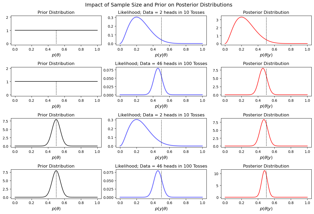
Bayesian update in action: The plot below illustrates the posterior distribution for a simple coin toss experiment across various sample sizes and with two distinct prior distributions. This visualization provides insights into how the combination of different sample sizes and prior beliefs influences the resulting posterior distributions.  

How to Model the Posterior Distribution

The seemingly simple posterior distribution in most cases is hard to compute. In particular, the denominator i.e. the marginal likelihood integral tends to be interactable, especially when working with a higher dimension parameter space. And in most cases there's no closed-form solution and numerical integration methods are also computationally intensive. To address this challenge we rely on a special class of algorithms called Markov Chain Monte Carlo simulations to model the posterior distribution. The idea here is to sample from the posterior distribution rather than explicitly modeling it and using those samples to represent the distribution of the model parameters

Markov Chain Monte Carlo (MCMC)

"MCMC methods comprise a class of algorithms for sampling from a probability distribution. By constructing a Markov chain that has the desired distribution as its equilibrium distribution, one can obtain a sample of the desired distribution by recording states from the chain" [3].  A few of the commonly used MCMC samplers are:

• Metropolis-Hastings
• Gibbs Sampler
• Hamiltonian Monte Carlo (HMC)
• No-U-Turn Sampler (NUTS)
• Sequential Monte Carlo (SMC)

Probabilistic Programming

Probabilistic Programming is a programming framework for Bayesian statistics i.e. it concerns the development of syntax and semantics for languages that denote conditional inference problems and develop "solvers” for those inference problems. In essence, Probabilistic Programming is to Bayesian Modeling what automated differentiation tools are to classical Machine Learning and Deep Learning models [2]. 

There exists a diverse ecosystem of Probabilistic Programming languages, each with its own syntax, semantics, and capabilities. Some of the most popular languages include:

• BUGS (Bayesian inference Using Gibbs Sampling) [4]: BUGS is one of the earliest probabilistic programming languages, known for its user-friendly interface and support for a wide range of probabilistic models. It implements Gibbs sampling and other Markov Chain Monte Carlo (MCMC) methods for inference.
• JAGS (Just Another Gibbs Sampler) [5]: JAGS is a specialized language for Bayesian hierarchical modeling, particularly suited for complex models with nested structures. It utilizes the Gibbs sampling algorithm for posterior inference.
• STAN: A probabilistic programming language renowned for its expressive modeling syntax and efficient sampling algorithms. STAN is widely used in academia and industry for a variety of Bayesian modeling tasks. "Stan differs from BUGS and JAGS  in two primary ways. First, Stan is based on a new imperative probabilistic programming language that is more flexible and expressive than the declarative graphical modeling languages underlying BUGS or JAGS, in ways such as declaring variables with types and supporting local variables and conditional statements. Second, Stan’s Markov chain Monte Carlo (MCMC) techniques are based on Hamiltonian Monte Carlo (HMC), a more efficient and robust sampler than Gibbs sampling or Metropolis-Hastings for models with complex posteriors" [6].
• BayesDB: BayesDB is a probabilistic programming platform designed for large-scale data analysis and probabilistic database querying. It enables users to perform probabilistic inference on relational databases using SQL-like queries [7]
• PyMC3: PyMC3 is a Python library for Probabilistic Programming that offers an intuitive and flexible interface for building and analyzing probabilistic models. It leverages advanced sampling algorithms such as Hamiltonian Monte Carlo (HMC) and Automatic Differentiation Variational Inference (ADVI) for inference [8].
• TensorFlow Probability: "TensorFlow Probability (TFP) is a Python library built on TensorFlow that makes it easy to combine probabilistic models and deep learning on modern hardware (TPU, GPU)" [9].
• Pyro: "Pyro is a universal probabilistic programming language (PPL) written in Python and supported by PyTorch on the backend. Pyro enables flexible and expressive deep probabilistic modeling, unifying the best of modern deep learning and Bayesian modeling" [10].
  

 These languages share a common workflow, outlined below:

1. Model definition: The model defines the processes governing data generation, latent parameters, and their interrelationships. This step requires careful consideration of the underlying system and the assumptions made about its behavior.
2. Prior distribution specification: Define the prior distributions for the unknown parameters within the model.  These priors encode the practitioner's beliefs, domain, or prior knowledge about the parameters before observing any data.
3. Likelihood specification: Describe the likelihood function, representing the probability distribution of observed data conditioned on the unknown parameters. The likelihood function quantifies the agreement between the model predictions and the observed data.
4. Posterior distribution inference: Use a sampling algorithm to approximate the posterior distribution of the model parameters given the observed data. This typically involves running Markov Chain Monte Carlo (MCMC) or Variational Inference (VI) algorithms to generate samples from the posterior distribution.

Case Study: Forecasting Stock Index Volatility 

In this case study, we will employ Bayesian modeling techniques to forecast the volatility of a stock index. Volatility here measures the degree of variation in a stock's price over time and is a crucial metric for assessing the risk associated with a particular stock.

Data: For this analysis, we will utilize historical data from the S&P 500 stock index. The S&P 500 is a widely used benchmark index that tracks the performance of 500 large-cap stocks in the United States. By examining the percentage change in the index's price over time, we can gain insights into its volatility. 

S&P 500 — Share Price and Percentage Change

From the plot above, we can see that the time series — price change between consecutive days has:

• Constant Mean
• Changing variance over time, i.e., the time series exhibits heteroscedasticity

Modeling Heteroscedasticity: "In statistics, a sequence of random variables is homoscedastic if all its random variables have the same finite variance; this is also known as homogeneity of variance. The complementary notion is called heteroscedasticity, also known as heterogeneity of variance" [11]. Auto-regressive Conditional Heteroskedasticity (ARCH) models are specifically designed to address heteroscedasticity in time series data.

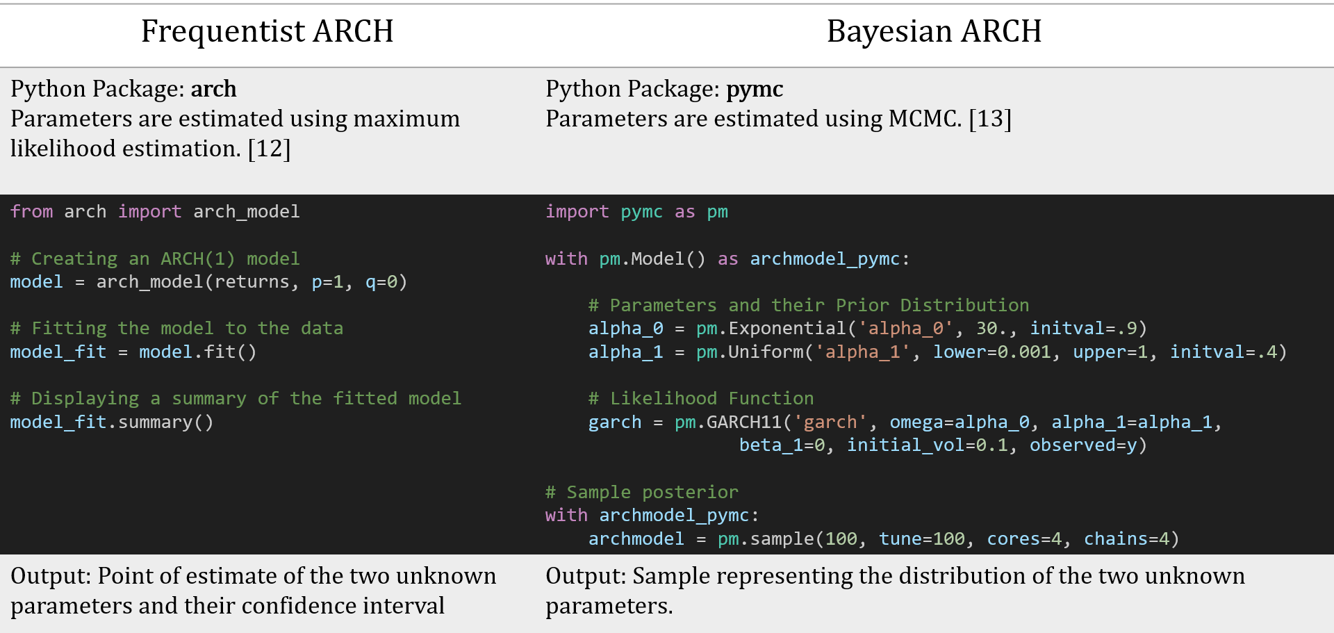
Bayesian vs. Frequentist Implementation of ARCH Model

The key benefits of Bayesian modeling include the ability to incorporate prior information and quantify uncertainty in model parameters and predictions. These are particularly useful in settings with limited data and when prior knowledge is available.

In conclusion, Bayesian modeling and probabilistic programming offer powerful tools for addressing the limitations of traditional machine-learning approaches. By embracing uncertainty quantification, incorporating prior knowledge, and providing transparent inference mechanisms, these techniques empower data scientists to make more informed decisions in complex real-world scenarios. 

References

1. Fornacon-Wood, I., Mistry, H., Johnson-Hart, C., Faivre-Finn, C., O'Connor, J.P. and Price, G.J., 2022. Understanding the differences between Bayesian and frequentist statistics. International journal of radiation oncology, biology, physics, 112(5), pp.1076-1082.
2. Van de Meent, J.W., Paige, B., Yang, H. and Wood, F., 2018. An Introduction to Probabilistic Programming. arXiv preprint arXiv:1809.10756.
3. Markov chain Monte Carlo 
4. Spiegelhalter, D., Thomas, A., Best, N. and Gilks, W., 1996. BUGS 0.5: Bayesian inference using Gibbs sampling manual (version ii). MRC Biostatistics Unit, Institute of Public Health, Cambridge, UK, pp.1-59.
5. Hornik, K., Leisch, F., Zeileis, A. and Plummer, M., 2003. JAGS: A program for analysis of Bayesian graphical models using Gibbs sampling. In Proceedings of DSC (Vol. 2, No. 1).
6. Carpenter, B., Gelman, A., Hoffman, M.D., Lee, D., Goodrich, B., Betancourt, M., Brubaker, M.A., Guo, J., Li, P. and Riddell, A., 2017. Stan: A probabilistic programming language. Journal of statistical software, 76.
7. BayesDB
8. PyMC
9. TensorFlow Probability
10. Pyro AI
11. Homoscedasticity and heteroscedasticity
12. Introduction to ARCH Models
13. pymc.GARCH11