Perceptron Explained Using Python Example - Data Analytics

In this post, you will learn about Perceptrons with the help of a Python example. It is very important for data scientists to understand the concepts related to Perceptron as a good understanding lays the foundation of learning advanced concepts of neural networks including deep neural networks (deep learning).

What Is a Perceptron?

Perceptron is a machine learning algorithm which mimics how a neuron in the brain works. It is also called as single layer neural network, as the output is decided based on the outcome of just one activation function which represents a neuron. 

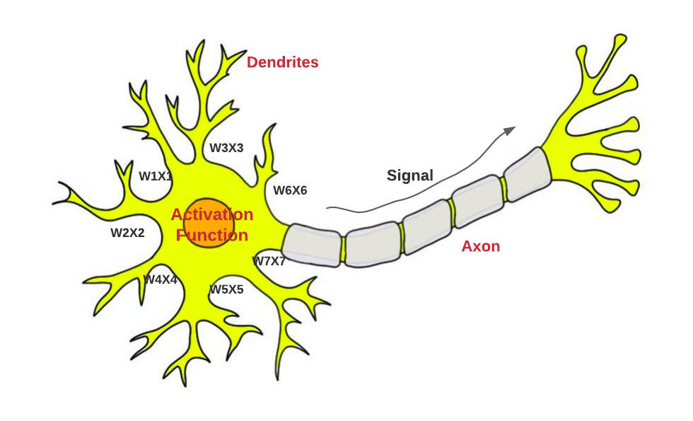
Let's first understand how a neuron works. The diagram below represents a neuron in the brain. The input signals (x1, x2, ...) of different strength (observe weights, w1, w2 ...) is fed into the neuron cell via dendrites. The net input (weighted sum) is processed by the neuron and output signal (observer signal in AXON) is appropriately fired. In case the combined signal strength is not appropriate based on decision function within neuron cell (observe activation function), the neuron does not fire any output signal.

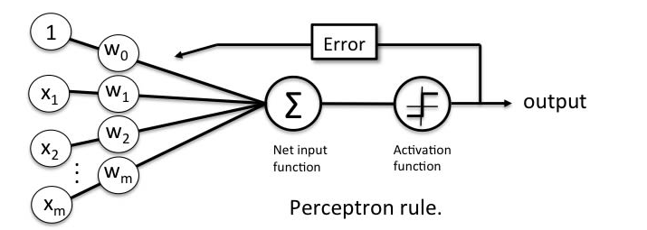
The perceptron when represented as a line diagram would look like the following:

Pay attention to some of the following in relation to what's shown in the above diagram representing a neuron:

• Step 1 - Input signals weighted and combined as net input: Weighted sums of input signal reaches the neuron cell through dendrites. The weighted inputs represent the fact that different input signal may have different strength, and thus, weighted sum. This weighted sum can as well be termed as net input to the neuron cell.
• Step 2 - Net input fed into activation function: Weighted The weighted sum of inputs or net input is fed as input to what is called as activation function.
• Step 3A - Activation function outputs binary signal appropriately: The activation function processes the net input based on unit step (heaviside) function and outputs the binary signal appropriately as either 1 or 0. The activation function for perceptron can said to be unit step function.
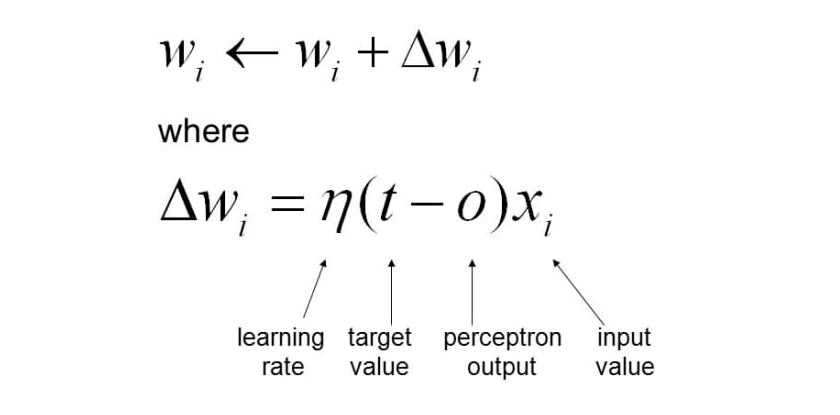
•  Step 3B - Learning input signal weights based on prediction vs actuals: A parallel step is neuron sending the feedback to strengthen the input signal strength (weights) appropriately such that it could create output signal appropriately that matches the actual value. The feedback is based on the outcome of the activation function which is a unit step function. Weights are updated based on the gradient descent learning algorithm. Here is my post on gradient descent - Gradient descent explained simply with examples. Here is the equation based on which the weights get updated:

Pay attention to some of the following in above equation vis-a-vis Perceptron learning algorithm:

• Weights get updated by \(\delta w\)
• \(\delta w\) is derived by taking first order derivative of loss function (gradient) and multiplying the output with negative (gradient descent) of learning rate. The output is what is shown in the above equation - product of learning rate, difference between actual and predicted value (perceptron output) and input value.
• In this post, the weights are updated based on each training example such that perceptron can learn to predict closer to actual output for next input signal. This is also called as stochastic gradient descent (SGD). Here is my post on stochastic gradient descent. That said, one could also try batch gradient descent to learn the weights of input signals.

Perceptron Python Code Example

In this section, we will look each of the steps described in previous section and understand the implementation with the Python code:

• Input signals weighted and combined as net input: Input signals get multiplied with weights and the sum of all weighted input signal is taken. This sum is called as net input and would be fed into activation function. Here is the code for net input. Note the dot product of coefficients with input X. Coefficient[0] is multiplied with 1 (bias element).

xxxxxxxxxx

'''

Net Input is sum of weighted input signals

'''

def net_input(self, X):

   weighted_sum = np.dot(X, self.coef_[1:]) + self.coef_[0]

   return weighted_sum

• Activation function invoked with net input: Net input is fed into activation function and output is determined based on the outcome of unit step function. Here is the code:

xxxxxxxxxx

'''

Activation function is fed the net input and the unit step function is executed to determine the output.

'''

def activation_function(self, X):

    weighted_sum = self.net_input(X)

    return np.where(weighted_sum >= 0.0, 1, 0)

• Prediction based on the activation function output: In Perceptron, the prediction output coincides with (or equal to ) the output of activation function which uses unit step function. This is where the Perceptron is different from ADAptive LInear NEuron also termed as Adaline. The Adaline algorithm implementation will be described in future post. In Adaline algorithm, the activation function is identity function and prediction is done based on unit step function output.

xxxxxxxxxx

'''

Prediction is made on the basis of output of activation function

'''

def predict(self, X):

    return self.activation_function(X)

• Learning weights based on the prediction vs actual: Weights are learned based on comparing the value of actual label and the predicted label (binary) and applying stochastic gradient descent algorithm to learn weights based on each training example. The idea is to improve on making predictions based on the learning from last training example. Here is the fit method which demonstrates the learning of input weights:

xxxxxxxxxx

'''

Stochastic Gradient Descent 

1. Weights are updated based on each training examples.

2. Learning of weights can continue for multiple iterations

3. Learning rate needs to be defined

'''

def fit(self, X, y):

    rgen = np.random.RandomState(self.random_state)

    self.coef_ = rgen.normal(loc=0.0, scale=0.01, size=1 + X.shape[1])

    for _ in range(self.n_iterations):

        for xi, expected_value in zip(X, y):

            predicted_value = self.predict(xi)

            self.coef_[1:] = self.coef_[1:] + self.learning_rate * (expected_value - predicted_value) * xi

            self.coef_[0] = self.coef_[0] + self.learning_rate * (expected_value - predicted_value) * 1

Here is how the entire Python code for Perceptron implementation would look like. This implementation is used to train the binary classification model that could be used to classify the data in one of the binary classes. Pay attention to all the methods that are explained previously. Also, pay attention to the score method which is used to measure the accuracy of the model.

xxxxxxxxxx

import numpy as np

#

# Perceptron implementation

#

class CustomPerceptron(object):

    def __init__(self, n_iterations=100, random_state=1, learning_rate=0.01):

        self.n_iterations = n_iterations

        self.random_state = random_state

        self.learning_rate = learning_rate

    '''

    Stochastic Gradient Descent 

    1. Weights are updated based on each training examples.

    2. Learning of weights can continue for multiple iterations

    3. Learning rate needs to be defined

    '''

    def fit(self, X, y):

        rgen = np.random.RandomState(self.random_state)

        self.coef_ = rgen.normal(loc=0.0, scale=0.01, size=1 + X.shape[1])

        for _ in range(self.n_iterations):

            for xi, expected_value in zip(X, y):

                predicted_value = self.predict(xi)

                self.coef_[1:] = self.coef_[1:] + self.learning_rate * (expected_value - predicted_value) * xi

                self.coef_[0] = self.coef_[0] + self.learning_rate * (expected_value - predicted_value) * 1

    '''

    Net Input is sum of weighted input signals

    '''

    def net_input(self, X):

            weighted_sum = np.dot(X, self.coef_[1:]) + self.coef_[0]

            return weighted_sum

    '''

    Activation function is fed the net input and the unit step function

    is executed to determine the output.

    '''

    def activation_function(self, X):

            weighted_sum = self.net_input(X)

            return np.where(weighted_sum >= 0.0, 1, 0)

    '''

    Prediction is made on the basis of output of activation function

    '''

    def predict(self, X):

        return self.activation_function(X) 

    '''

    Model score is calculated based on comparison of 

    expected value and predicted value

    '''

    def score(self, X, y):

        misclassified_data_count = 0

        for xi, target in zip(X, y):

            output = self.predict(xi)

            if(target != output):

                misclassified_data_count += 1

        total_data_count = len(X)

        self.score_ = (total_data_count - misclassified_data_count)/total_data_count

        return self.score_

Here is the Python code which could be used to train the model using CustomPerceptron algorithm shown above. Note that SKlean breast cancer data is used for training the model in order to classify / predict the breast cancer.

xxxxxxxxxx

import numpy as np

from sklearn import datasets

from sklearn.model_selection import train_test_split

#

# Load the data set

#

bc = datasets.load_breast_cancer()

X = bc.data

y = bc.target

#

# Create training and test split

#

X_train, X_test, y_train, y_test = train_test_split(X, y, test_size=0.3, random_state=42, stratify=y)

#

# Instantiate CustomPerceptron

#

prcptrn = CustomPerceptron()

#

# Fit the model

#

prcptrn.fit(X_train, y_train)

#

# Score the model

#

prcptrn.score(X_test, y_test), prcptrn.score(X_train, y_train)

Conclusions

Here is the summary of what you learned about the Perceptron algorithm with help of Python implementation:

• Perceptron mimics the neuron in the human brain
• Perceptron is termed as machine learning algorithm as weights of input signals are learned using the algorithm
• Perceptron algorithm learns the weight using gradient descent algorithm. Both stochastic gradient descent and batch gradient descent could be used for learning the weights of the input signals
• The activation function of Perceptron is based on the unit step function which outputs 1 if the net input value is greater than or equal to 0, else 0.
• The prediction is also based on the unit step function.