Next-Gen Data Pipes With Spark, Kafka and k8s

Introduction

Data integration has always played an essential role in the information architecture of any enterprise. Specifically, the analytical processes of the enterprise heavily depend on this integration pattern in order for the data to be made available from transactional systems and loaded in an analytics-friendly format. When the systems were not interconnected so much in the traditional architecture paradigm, and the latency between transactions and analytical insights was permissible and the integrations mainly were batch-oriented. 

In the batch pattern, typically, large files (data dump) are generated by the operational systems, and those are processed (validated, cleansed, standardized, and transformed) to create some output files to feed to the analytical systems. Of course, reading such large files was memory intensive; hence, data architects used to rely upon a series of staging databases to store step-by-step data processing output.  As the distributed computing evolved to Hadoop, MapReduce addressed the high memory requirement by distributing the processing across horizontally scalable commoditized hardware. As the computing technique has evolved further, it is now possible to run MapReduce in-memory, which today has become a kind of de-facto standard for processing large data files. 

While the batch processing was going through a process of evolution, there has also been significant development on the non-batch side. Over the years, user-facing IoT devices became part of operational systems, web feeds an essential source of data, and event-driven architecture became a popular choice in the microservice-based cloud-native development approach. In this changed scenario, the frequency of data processing increased manifold, and the ability to process data stream became the primary non-functional requirement for the data integration jobs.  As a result, data integration, which was once a large file processing problem, has currently evolved to a stream processing problem, calling for a good data pipe with sufficient buffer so that data packets are not lost and becomes durable. 

Since cloud is the platform of choice today, horizontal scaling is preferred over the vertical one in any component that we design. As a result, there is a definite lookout of horizontal scalability of the stream as well as the consumer of the stream. This is where some promises are observed to run streaming solutions, such as Kafka, as well as consumer on Kubernetes cluster. It is believed that this would possibly be the most widely accepted trend in the speed layer of Lambda architecture as well as building Kappa architecture. 

This article talks about the architecture patterns along with some sample code for the readers to implement them in their own environment.

Lambda Architecture

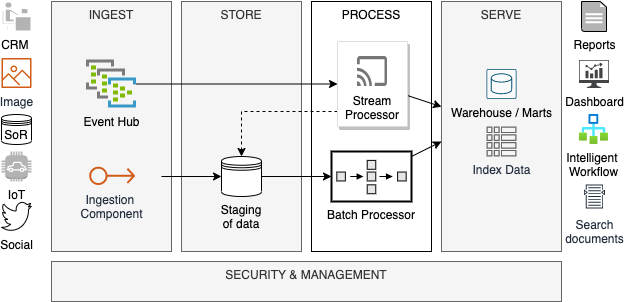
In Lambda Architecture, there are two main layers – Batch and Speed. The first one transforms data in scheduled batches whereas the second is responsible for near real-time data processing. The batch layer is typically used when the source system sends the data in batches, access to the entire dataset is needed for required data processing, or the dataset is too large to be handled as a stream. On the contrary, stream processing is needed for small packets of high-velocity data, where the packets are either mutually independent or packets in close vicinity form a context. Naturally, both types of data processing are computation-intensive, though the memory requirement for batch is higher than the stream layer. Architects look for solution patterns that are elastic, fault-tolerant, performing, cost-effective, flexible, and, last but not least – distributed. 

As evident from the diagram above, Lambda architecture is complex because it has two separate components for handling batch and stream processing of data. The complexity can be reduced if one single technology component can serve both purposes. Apache Spark has some promising features in this regard, which we will see in subsequent section of this article.  

Recent Options in Distributed Computing

With its array of libraries, including Spark SQL and Spark Streaming, Apache Spark appears as a very potent solution implementing distributed Lambda architecture with in-memory computing. Spark SQL supports all batch operations such as loading of data, validation, transformation, aggregation, and mapping through a distributed architecture that reduces the memory requirement of any individual machine. Similarly, Spark Streaming-based jobs can process data on a near real-time basis from sources like Kafka streams and feed the insights to more durable components like a data warehouse or data lake.

Kubernetes is the de-facto cluster manager in cloud platforms, and the latest version of Spark can run on a cluster managed by Kubernetes. Therefore, Spark on Kubernetes is an excellent combination for implementing Lambda architecture on the cloud. 

One can use Kubernetes alone for distributed computing, but we need to rely on custom solutions in such cases. For example, in the case of the batch layer, “Spring batch” framework can be used in conjunction with the Kubernetes cluster for distributing the work to multiple cluster nodes. Similarly, Kubernetes can distribute stream data to several pods that run in parallel for the speed layer. The pods can scale horizontally at ease by spawning the containers within them, and then the cluster can be adjusted based on the volume and velocity of the data. 

Spark - One Stop Solution for Lambda Architecture

Apache Spark scores quite well as far as the non-functional requirements of batch and speed layers are concerned:

• Scalability: Spark the cluster can be scaled up or down based on requirements. It consists of a master node with a set of worker nodes that adds horizontal scalability with increasing workload.
• Fault tolerance: In any of the worker node crashes causing fault in the cluster, Spark framework takes care of it. Each data frame is logically partitioned and data processing of each partition happens on a certain node. While processing data, if any of the node fails then Cluster Manager assigns another node to execute the same partition of the data frame by following DAG (Directed Acyclic Graph), which ensures absolutely zero data loss.
• Performance: As Spark supports in-memory computation, data can be stored in RAM during execution instead of disks (as needed for Hadoop), which makes it a lot faster option. 
• Flexible workload distribution: Since Spark supports distributed computing, it shares components of a task across multiple nodes and generates output as an ensemble unit. Spark can run on the cluster managed by Kubernetes, which makes it even more appropriate choice in cloud environment.
• Cost: Spark is open-source and does not include any cost itself. Of course, if managed services are opted for, those come with a cost. 

Let us now deep dive a bit into Spark to understand how it helps in batch and steam processing. Spark consists of two main components: Spark core API and Spark libraries. Core API layer provides support for four languages: R, Python, Scala, and Java. On top of Core API layer, we have the following Spark libraries, each aimed for different purposes.

• Spark SQL: handles (semi-)structured data, performs basic transformation functions and execute SQL queries on datasetSpark Streaming: capable of handling stream data; supports near real-time data processing
• Spark MLib: used for machine learning; to be used for data processing on a need-basis 
• Spark GraphX: used for graph processing; very little usage for the scope discussed here 

Spark for Batch Layer

In the batch layer of Lambda architecture transformation, calculation, aggregation operations over (semi-)structured data are handled by Spark SQL Library. Let us further discuss Spark SQL architecture. 

As evident from the diagram above, Spark SQL has three main architectural layers as explained below:

• Datasource API: This handles different data formats like CSV, JSON, AVRO and PARQUET. It also helps to connect different data sources like HDFS, HIVE, MYSQL, CASSANDRA etc. Common APIs to load data from different formats as: 

Dataframe.read.load(“ParquetFile | JsonFile | TextFile | CSVFile | AVROFile”)

• Dataframe API: Spark 2.0 onwards, Spark dataframes are being largely used. It helps to hold large relational data and expose multiple transformational function to slice and dice the dataset. Examples of such transformational functions exposed through Dataframe API are:  

withColumn, select, withColumnRenamed, groupBy, filter, sort, orderBy etc.

• SQL service: Spark SQL Service is the main element which helps us to create dataframe and hold relational data for further transformation. This is the entry point for transformation in batch layer when we use Spark SQL. During transformation, different APIs can be used in python, R, Scala or Java and also SQL can be executed directly to transform the data.

Below are some examples of code for batch processing: 

Suppose there are two tables: one is PRODUCT, and another is TRANSACTION. PRODUCT table consists of all the information about specific products of a store, and Transaction table consists of all the transaction made against each product. We can get the following information by using transformation and aggregation. 

• Product wise total quantity sold
• Segment wise total revenue earned

The same result can be obtained by writing plain SQL on the spark dataframe or by using aggregation functions.

from pyspark.sql import SparkSession
from pyspark.sql.functions import *

spark = SparkSession.builder.master("local").appName("Superstore").getOrCreate()
df1 = spark.read.csv("Product.csv")
df2 = spark.read.csv("Transaction.csv")
df3 = df1.filter(df1.Segment != 'Electric')
df4 = df2.withColumn("OrderDate",df2.OrderDate[7:10])

result_df1 = df3.join(df4, on= ['ProductCode'], how='inner')

result_df2 = result_df1.groupBy('ProductName').sum('Quantity')
result_df2.show()

# Display segment wise revenue generated
result_df3 = result_df1.groupBy('Segment').sum('Price')
result_df3.show()

from pyspark.sql import SparkSession
from pyspark.sql.functions import *

spark = SparkSession.builder.master("local").appName("Superstore").getOrCreate()
df1 = spark.read.csv("Product.csv")
df2 = spark.read.csv("Transaction.csv")
df3 = df1.filter(df1.Segment != 'Electric')
df4 = df2.withColumn("OrderDate",df2.OrderDate[7:10])

result_df1 = df3.join(df4, on= ['ProductCode'], how='inner')
result_df1.createOrReplaceTempView("SuperStore")

# Display product wise quantity sold
result_df2 = spark.sql("select ProductName , Sum(Quantity) from Superstore group by ProductName")
result_df2.show()

# Display segment wise revenue earned
result_df3 = spark.sql("select Segment , Sum(Price) from Superstore group by Segment")
result_df2.show()

In both cases, the first data is loaded from two different sources, and Product data is filtered for all the non-electrical products. Transaction data is altered based on a certain format of order date. Then, both dataframes are joined and produce results for segment-wise revenue earned and product-wise quantity sold in this superstore. 

This is, of course, a simple example of loading, validation, transformation, and aggregation. More complex operations are possible with Spark SQL. To know more about Spark SQL services, refer to the documentation here.

Spark for Speed layer

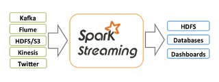
Spark Streaming is a library, used on top of core spark framework. It ensures scalability, high-throughput, and fault tolerance for live data stream processing.

Figure 5: Spark Streaming architecture (source: https://spark.apache.org)

As shown in the diagram above, Spark converts input data stream to batches of input data. There are two implementations of such discrete batches: a) Dstreams or Discretized Streams and b) Structured Streaming. The former was very popular until the latter came in as a more advanced version. However, Dstream is not completely obsolete yet and is kept in this article for completeness. 

• Discretized Streams: This provides an abstraction over spark streaming library. It is a collection of RDDs and represents a continuous stream of data. It discretizes data into tiny batches and runs small jobs to process those tiny batches. Tasks are assigned to the worker node based on the location of the data. So, by this concept of Dstream, spark can read data parallelly, executing tiny batches to process the stream and ensure efficient node allocation for the stream processing.
• Structured Streaming: This is the most advanced and modern approach of stream processing by using spark engine. It is well integrated with Spark Dataframe API (discussed in the section above for batch processing) for all kinds of operations over stream data. Structured Streaming can process data incrementally and continuously. Near real-time aggregation is also possible based on a certain window and watermark.

There can be different stream processing use cases that can be handled by spark structured streaming, as shown in the examples given below:

Simple Structured Streaming 

Simple structured streaming will only transform and load data from streams and does not include any aggregation over a specific time frame. As for example, a system takes data from Apache Kafka and transforms it in near real-time basis by spark streaming and Spark SQL (see the code snippet below).

from pyspark.sql import SparkSession
from pyspark.streaming import StreamingContext
import pyspark.sql.functions as sf

spark=SparkSession.builder.master('local').appName('StructuredStreamingApp').getOrCreate()
df = spark.readStream.format("kafka").option("kafka.bootstrap.servers,"localhost:9092")
                                             .option("subscribe", "test_topic").load()
df1 = df.selectExpr("CAST(value AS STRING)")
df2 = df1.selectExpr("split(value, ',')[0] as Dept","split(value, ',')[1] as Age")
df2.show()

The ReadStream function of the Spark Session object is used to connect a specific Kafka topic.  As in the above code snippet within the options, we need to provide the IP of the Kafka cluster broker and Kafka topic name. The output of this code is a table, having two columns: Dept and Age.

Aggregation on Structured Streaming

Aggregation can be done on the streaming data by Structured Streaming, which is able to calculate the rolling aggregation results on top of the arrival of the new events. This is the running aggregation on the whole data stream. Please refer to the code snippet below, which derives department wise average age on whole data stream.

from pyspark.sql import SparkSession
from pyspark.streaming import StreamingContext
import pyspark.sql.functions as sf

spark=SparkSession.builder.master('local').appName('StructuredStreamingApp').getOrCreate()
df = spark.readStream.format("kafka").option("kafka.bootstrap.servers", "localhost:9092")
                                     .option("subscribe", "test_topic").load()
df1 = df.selectExpr("CAST(value AS STRING)")
df2 = df1.selectExpr("split(value, ',')[0] as Dept","split(value, ',')[1] as Age")
df3 = df2.groupBy("Dept").avg("Age")
df3.show()

Aggregation on Window

Sometimes we need aggregation over a certain window of time instead of running aggregation. Spark Structured Streaming also provides such a facility. Suppose we want to count the number of events in the last 5 mins.  This Window function with aggregation will help us.

from pyspark.sql import SparkSession
from pyspark.streaming import StreamingContext
import pyspark.sql.functions as sf
import datetime
import time

spark=SparkSession.builder.master('local').appName('StructuredStreamingApp').getOrCreate()
df = spark.readStream.format("kafka").option("kafka.bootstrap.servers", "localhost:9092")
                                     .option("subscribe", "test_topic").load()
df1 = df.selectExpr("CAST(value AS STRING)")
df2 = df1.selectExpr("split(value, ',')[0] as Dept","split(value, ',')[1] as Age")
df3 = df2.withColumn("Age", df2.Age.cast('int'))
df4 = df3.withColumn("eventTime",sf.current_timestamp())
df_final = df4.groupBy(sf.window("eventTime", "5 minute")).count()
df_final.show()

Aggregation on overlapping window 

In the above example, each window is a group for which aggregation is done. There is also a provision to define an overlapping window by mentioning window length and sliding interval. It is very useful in late data handling in windowed aggregation. The code below calculates the number of events based on a 5-minute window, having a sliding interval of 10 minutes.

from pyspark.sql import SparkSession
from pyspark.streaming import StreamingContext
import pyspark.sql.functions as sf
import datetime
import time

spark=SparkSession.builder.master('local').appName('StructuredStreamingApp').getOrCreate()
df = spark.readStream.format("kafka").option("kafka.bootstrap.servers", "localhost:9092")
                                     .option("subscribe", "test_topic").load()
df1 = df.selectExpr("CAST(value AS STRING)")
df2 = df1.selectExpr("split(value, ',')[0] as Dept","split(value, ',')[1] as Age")
df3 = df2.withColumn("Age", df2.Age.cast('int'))
df4 = df3.withColumn("eventTime",sf.current_timestamp())
df_final = df4.groupBy("Dept",sf.window("eventTime","10 minutes", "5 minute")).count()
df_final.show()

Aggregation with watermarking and overlapping window

Late arrival of data creates a problem in aggregation of near real-time systems. We can use overlapping window to solve this error. But the question is: how much time will the system wait for late data? This can be resolved through watermarking. By this approach, we define a certain period on top of overlapping window.  After that, the system discards the event.

from pyspark.sql import SparkSession
from pyspark.streaming import StreamingContext
import pyspark.sql.functions as sf
import datetime
import time
spark=SparkSession.builder.master('local').appName('StructuredStreamingApp').getOrCreate()
df = spark.readStream.format("kafka").option("kafka.bootstrap.servers", "localhost:9092")
                                     .option("subscribe", "test_topic").load()
df1 = df.selectExpr("CAST(value AS STRING)")
df2 = df1.selectExpr("split(value, ',')[0] as Dept","split(value, ',')[1] as Age")
df3 = df2.withColumn("Age", df2.Age.cast('int'))
df4 = df3.withColumn("eventTime",sf.current_timestamp())
df_final = df4.withWatermark("eventTime","10 Minutes").groupBy("Dept",sf.window("eventTime","10 minutes", "5 minute")).count()
df_final.show()

The code above indicates that for late events, after 10 mins, the old window result will not be updated.

Kafka + k8s - Another Solution for Speed Layer

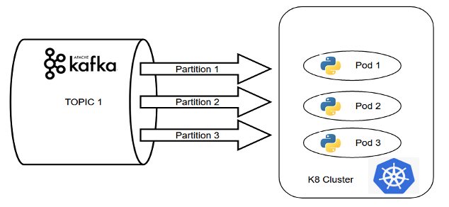
Pods hosted on Kubernetes cluster, forming a consumer group for Kafka stream, is another approach for near real-time data processing. By using this combination, we can easily get the advantages of distributed computing. 

In the event driven system in the above example, data is being loaded into the python-based processing unit from Kafka topic. If the number of partitions in the Kafka cluster matches with the replication factor of the pods, the pods together form a consumer group and the messages are consumed in a seamless manner. 

This is a classic example of building a distributed data processing system which ensures parallel processing by only using Kafka + k8s combination. 

Two very popular libraries to create Kafka consumer by using python are:

• Python_Kafka Library
• Confluent_Kafka Library

Python_Kafka

from kafka import KafkaConsumer

consumer = KafkaConsumer(TopicName,
                         bootstrap_servers= <broker-list>,
                         group_id=<GroupName>,
                         enable_auto_commit=True,
                         auto_offset_reset='earliest')

consumer.poll()

Confluent_Kafka 

from confluent_kafka import Consumer

consumer = Consumer({'bootstrap.servers': <broker-list>,
                     'group.id': <GroupName>,
                     'enable.auto.commit': True,
                     'auto.offset.reset': 'earliest'
                     })

consumer.subscribe([TopicName])

A sample structure of K8.yml file is as follows:

metadata:
  name: <app name>
  namespace: <deployment namespace>
  labels:
    app: <app name>
spec:
  replicas: <replication-factor>
  spec:
      containers:
      - name: <container name>

If the basic components are developed in the above manner, the system will get the help of distributed computing without in-memory computation. Everything depends upon volumetrics and desired speed of the system. For low/medium volume of data, one can ensure good speed by implementing this python-k8 based architecture.

Both of the approaches can be hosted in cloud with a variety of services. For example, we have EMR and Glue in AWS, spark cluster can be created by Dataproc in GCP, or we can use Databricks in Azure. On the other hand, the kafka-python-k8 approach can be easily implemented in cloud, which ensures better manageability.  For example in AWS, we can use the combination of MSK or Kinesis and EKS for this approach. In the next version, we will discuss the implementation of both batch and speed layers within all the cloud vendors, and also provide a comparison study on the basis of different requirements.