An Introduction to Linear Programming: Concepts, Formulation, and Solution Methods

Linear programming is a mathematical technique used to determine the optimal outcome — such as maximizing profit or minimizing cost — in a model where both the objective function and the constraints are expressed as linear relationships.

The term "programming" in linear programming originates from military terminology, referring to the process of planning schedules, such as coordinating supply lines or deploying units efficiently.

Key Concepts

Decision Variables

Decision variables are the core components of an optimization problem, representing quantities that can be adjusted to find the optimal solution that maximizes or minimizes the objective function while satisfying the constraints.

Objective Function

The objective function is a mathematical expression that defines the goal of the optimization problem. In linear programming, the objective function is always a linear combination of the decision variables.

Constraints

Constraints are the requirements that the solution to the optimization problem must satisfy. They are expressed as linear inequalities or equations involving the decision variables. Constraints can arise from various sources, such as resource availability, budget limitations, time restrictions, or physical laws. In a linear programming problem, constraints can be categorized as follows:

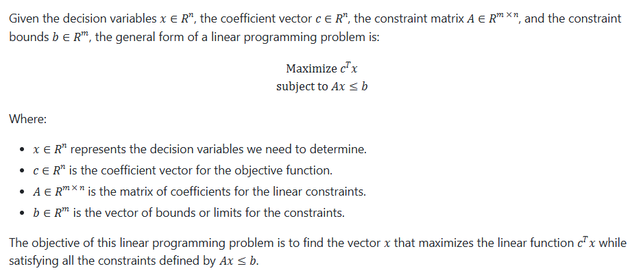
• Inequality Constraints: These specify that a certain relationship must hold, such as Ax ≤ b where A is a matrix of coefficients, x is the vector of decision variables, and b is a vector of constants.
•  Equality Constraints: These require that a particular relationship must be exact, expressed as Ax = b.

Feasible Region

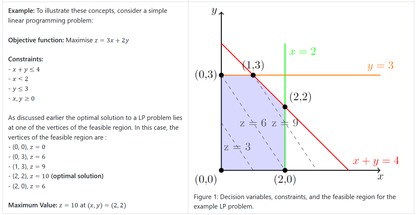
The feasible region is the set of all possible points (or vectors) that satisfy the constraints. Geometrically, this region is often represented as a convex polygon (or polyhedron in higher dimensions) in the space defined by the decision variables.

Fundamental Theorem of Linear Programming

"The fundamental theorem of linear programming (LP) states that every feasible linear program that is bounded below has an optimal solution in a zero-dimensional face (a vertex) of the feasible polyhedron" [1]. This means that the maximum or minimum of the objective function always occurs at the vertices of the feasible region. Additionally, this implies that an LP optimization problem may lack an optimal solution under the following circumstances [2]:

• There is no feasible region: If the inequality constraints are incompatible, no region in the graph will satisfy all constraints.
• The feasible region is unbounded: When the region extends infinitely, the linear program may not have a finite optimal solution.

Mathematical Formulation of LP Problem

Duality Problem

The duality theorem in linear programming states that any minimization problem can be transformed into an equivalent maximization problem, known as the dual problem, and vice versa. The minimum value of the objective function in the primal problem is achieved if and only if the maximum value of the objective function in its dual problem is also achieved. This relationship between primal and dual problems is key to understanding LP's duality theory, which provides a deeper insight into optimization problems.

Solving the dual problem can often be advantageous, particularly when the primal problem has a significantly larger number of constraints compared to decision variables. This is because the computational complexity of solving a linear programming problem typically increases more rapidly with the number of constraints than with the number of variables. In such cases, the dual problem, which has fewer constraints and more variables, can be solved more efficiently.

Solving Linear Programming Problems

LP problems can be solved using various methods, depending on the problem's complexity and dimensionality. These methods range from simple graphical methods to advanced computational algorithms.

Graphical Method

The Graphical Method, as demonstrated in the previous example, is one of the simplest approaches to solving linear programming problems, but it is limited to cases with two variables. The steps involved are as follows:

• Graph the constraints and feasibility region: The inequalities are plotted as straight lines, defining the feasible region where all constraints are satisfied.
• Objective function optimization: The objective function is maximized or minimized by evaluating its value at the vertices of the feasible region.

Simplex Method

The Simplex Method is an iterative algorithm that starts at one of the vertices of the feasible region and moves to an adjacent vertex that offers the greatest improvement to the objective function relative to the current vertex. The algorithm continues this process until it reaches the optimal solution, which occurs when it arrives at a vertex where all neighboring vertices either yield worse objective values or are outside the feasible region.

Ellipsoid Method

The Ellipsoid Method is an interior-point algorithm used to solve linear programming problems. Unlike the Simplex method, which operates on the vertices of the feasible region, the Ellipsoid Method works with the interior of the feasible region. It starts with an initial ellipsoid that encapsulates the entire feasible region and refines this ellipsoid at each step. By iterating through linear inequality constraints, the method progressively reduces the ellipsoid’s volume, bringing it closer to the optimal solution.

In terms of theoretical performance, the Ellipsoid Method is guaranteed to run in polynomial time, while the Simplex method, in contrast, can exhibit exponential time complexity in the worst case. This makes the Ellipsoid Method an appealing choice for large-scale problems in theory, although practical use has been limited by slower convergence compared to other methods, such as Interior-Point Methods [3].

Interior-Point Methods

Interior-point methods approach the optimal solution from within the feasible region rather than moving along the edges like the Simplex Method. They are more efficient for large-scale problems. These methods solve LP problems by following a trajectory through the interior of the feasible region, aiming to reach the optimal point directly. In contrast, the Simplex Method’s trajectory moves along the boundary, while the Ellipsoid Method encircles the feasible region from the outside [3]. Interior-point methods are particularly effective for large-scale optimization problems, as they exhibit more favorable performance than the Simplex Method, especially when dealing with very high-dimensional problems.

Application of LP Problems

Optimal Transport

A fundamental challenge in statistics and machine learning is developing effective measures of "distance" between pairs of probability distributions. A valid distance function should satisfy key properties, such as symmetry and triangle inequality. However, many common measures used to compare probability distributions fail to meet these criteria and are therefore classified as divergences (such as the Kullback-Leibler (KL) divergence) [4].

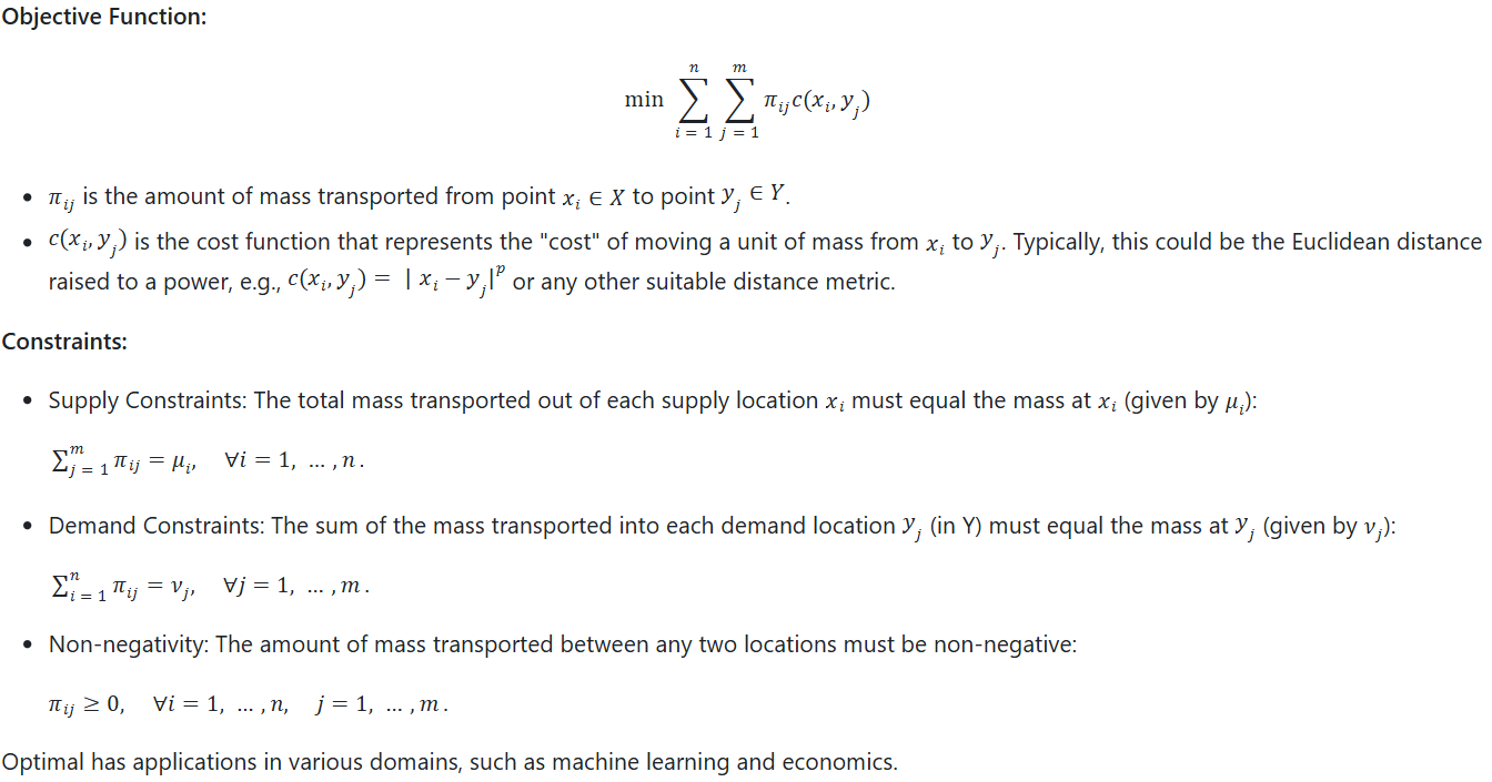
Optimal transport provides a robust distance measure between probability distributions. The intuition behind optimal transport is to imagine using a pile of dirt to fill a hole of the same volume at minimum cost. In other words, it seeks the most efficient way to move mass from one probability distribution X to another distribution Y while minimizing the transportation cost.

This can be framed as an LP problem:

Network Flow Problems

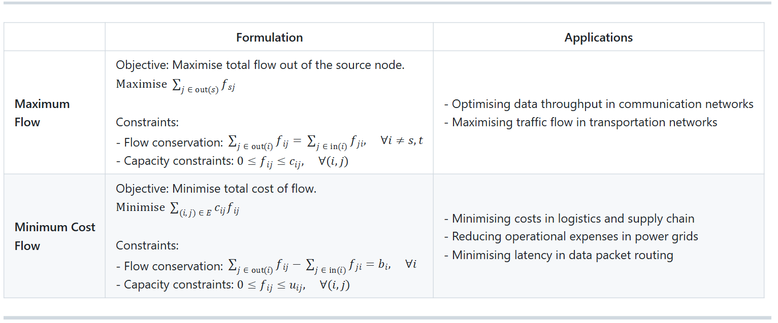
Network flow problems are integral to optimizing resource movement through networks, where resources may represent goods, data, or other commodities. These problems typically involve a directed graph in which each edge has a specified capacity and cost. The objective is to optimize the flow of resources from a source node to a sink node, subject to constraints on the edges and nodes. Key types of network flow problems include the Maximum Flow Problem, the Minimum Cost Flow Problem, etc. [5].

Libraries for Solving Linear Programming Problems

OR-Tools (Google) [6]: An open-source software suite developed by Google that supports LP and other constraint programming. It is highly scalable and integrates with several programming environments.

POT (Python Optimal Transport) [7]: A Python library specifically designed for solving Optimal Transport problems. It supports multiple solvers for OT, including LP-based methods, and is widely used in machine learning, statistics, and data science for tasks like domain adaptation, clustering, and generative modeling.

Conclusion

Linear programming remains a cornerstone of optimization, offering tools to address diverse problems in fields like logistics, finance, and AI. By mastering LP concepts and methods, practitioners can effectively solve both theoretical and real-world challenges.

References

 1. Tardella, F. (2010) ‘The fundamental theorem of linear programming: extensions and applications’, Optimization, 60(1–2), pp. 283–301. doi: 10.1080/02331934.2010.506535.

2. Sekhon, R., & Bloom, R. (2024). Applied finite mathematics.

3. Adams, S., 2020. MATH 510 Fall 2020.

4. Williams, A.H. (2020) Optimal Transport.

5. Wikipedia contributors. (2024). Network flow problem.

6. Google Developers, 2024. Google OR-Tools: Operations Research Tools.

7. Flamary, R. and Courty, N., 2024. POT: Python Optimal Transport Library.