XGBoost: A Deep Dive Into Boosting

Every day we hear about the breakthroughs in artificial intelligence. However, have you wondered what challenges it faces?

Challenges occur in highly unstructured data like DNA sequencing, credit card transactions, and even in cybersecurity, which is the backbone of keeping our online presence safe from fraudsters. Does this thought make you yearn to know more about the science and reasoning behind these systems? Do not worry! We’ve got you covered. In the cyber era, machine learning (ML) has provided us with the solutions to these problems with the implementation of Gradient Boosting Machines (GBM). We have ample algorithms to choose from to do gradient boosting for our training data but still, we encounter different issues like poor accuracy, high loss, large variance in the result. 

Here, we are going to introduce you to a state of the art machine learning algorithm XGBoost built by Tianqi Chen, that will not only overcome the issues but also perform exceptionally well for regression and classification problems. This blog will help you discover the insights, techniques, and skills with XGBoost that you can then bring to your machine learning projects.

XGBoost a Glance!

eXtreme Gradient Boosting (XGBoost) is a scalable and improved version of the gradient boosting algorithm (terminology alert) designed for efficacy, computational speed, and model performance. It is an open-source library and a part of the Distributed Machine Learning Community. XGBoost is a perfect blend of software and hardware capabilities designed to enhance existing boosting techniques with accuracy in the shortest amount of time. Here’s a quick look at an objective benchmark comparison of XGBoost with other gradient boosting algorithms trained on random forest with 500 trees, performed by Szilard Pafka.

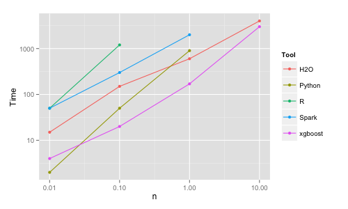
Benchmark Performance of XGBoost

A Quick Flashback to Boosting

Boosting generally means increasing performance. In ML, boosting is a sequential ensemble learning technique (another terminology alert, fret not! We will explain this as well) to convert a weak hypothesis or weak learners into strong learners to increase the accuracy of the model.

We can understand the need for boosting through a simple classification example: To classify a Twitter account as bot or human with the help of underlying rules (limited in extent):

RULES:

• No account information and profile photo → Bot
• Username is gibberish → Bot
• Tweeting in more than one language → Bot
• It has an adequate amount of activity and a profile→ Human
• An enormous amount of tweets per day → Bot
• Other accounts linked → Human

As now we are aware of the rules, let’s apply these on the below example:
Scenario — An account posting tweets in English and French.

The 3rd rule will classify it as a bot, but this will be a false prediction as a person can know and tweet in multiple languages. Consequently, based on a single rule, our prediction can be flawed. Since these individual rules are not strong enough to make an accurate prediction, they are called weak learners. Technically, a weak learner is a classifier that has a weak correlation with the actual value. Therefore, to make our predictions more accurate, we devise a model that combines weak learners’ predictions to make a strong learner, and this is done using the technique of boosting.

Weak rules are generated at each iteration by base learning algorithms which in our case can be of two types:

• Tree as base learner
• Linear base learner

Generally, decision trees are default base learners for boosting.

Interested to know more about learners? Be assured, we will demonstrate how to use both the base learners to train XGBoost models in a later section.

First, let’s get to know about the ensemble learning technique mentioned above.

Ensemble Learning

Ensemble learning is a process in which decisions from multiple machine learning models are combined to reduce errors and improve prediction when compared to a single ML model. Then the maximum voting technique is used on aggregated decisions (or predictions in machine learning jargon) to deduce the final prediction. Puzzled?

Think of it as organizing efficient routes to your work/college/or grocery stores. As you can use multiple routes to reach your destination, you tend to learn the traffic and the delay it might cause to you at different times of the day, allowing you to devise a perfect route, Ensemble learning is alike!

This image shows a clear distinction of a single ML model with respect to Ensemble Learner:

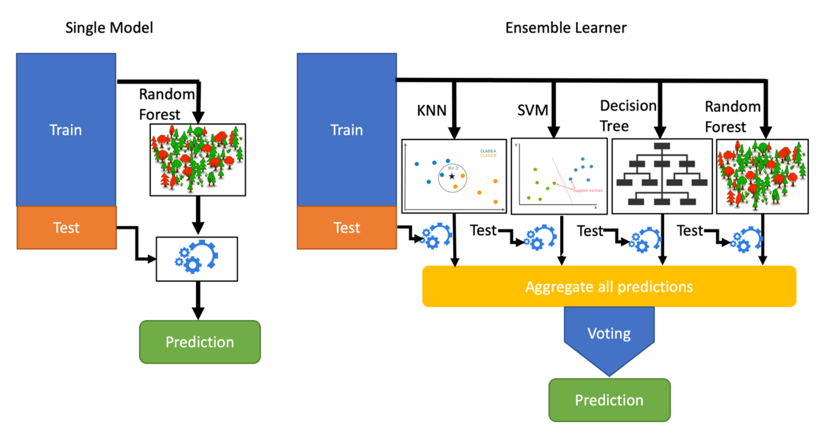
Single Model Prediction vs Ensemble Learner

Types of Ensemble learning:

Ensemble learning methods can be performed in two ways:

• Bagging (parallel ensemble)
• Boosting (sequential ensemble)

Though both have some fascinating math under the cover, we do not need to know it to be able to pick it up as a tool. Our focus will be more on the understanding of Boosting due to its relevance in XGBoost.

Working of Boosting Algorithm:

The boosting algorithm creates new weak learners (models) and sequentially combines their predictions to improve the overall performance of the model. For any incorrect prediction, larger weights are assigned to misclassified samples and lower ones to samples that are correctly classified. Weak learner models that perform better have higher weights in the final ensemble model. 

Boosting never changes the previous predictor and only corrects the next predictor by learning from mistakes. Since Boosting is greedy, it is recommended to set a stopping criterion such as model performance (early stopping) or several stages (e.g. depth of tree in tree-based learners) to prevent overfitting of training data. The first implementation of boosting was named AdaBoost (Adaptive Boosting).

  F(i) is current model, F(i-1) is previous model and f(i) represents weak 

model  

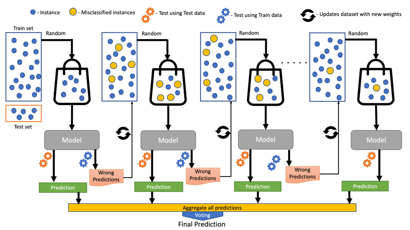
Internal working of boosting algorithm

Feeling braced up? Take a look at two more algorithms (CART and Gradient Boosting) to understand the mechanics of XGBoost before we delve deeper into the topic.

Classification and Regression Trees (CART):

A decision tree is a supervised machine learning algorithm used for predictive modeling of a dependent variable(target) based on the input of several independent variables. It has a tree-like structure with the root at the top. CART which stands for Classification and Regression Trees is used as an umbrella term to refer to the following types of decision trees:

Classification Trees: where the target variable is fixed or categorical, this algorithm is used to identify the class/category within which the target would most likely fall.

Regression Trees: where the target variable is continuous and the tree/algorithm is used to predict its value, e.g. predicting the weather.

Gradient Boosting:

Gradient boosting is a special case of boosting algorithm where errors are minimized by a gradient descent algorithm and produce a model in the form of weak prediction models e.g. decision trees.

The major difference between boosting and gradient boosting is how both the algorithms update model (weak learners) from wrong predictions. Gradient boosting adjusts weights by the use of gradient (a direction in the loss function) using an algorithm called Gradient Descent, which iteratively optimizes the loss of the model by updating weights. Loss normally means the difference between the predicted value and actual value. For regression algorithms, we use MSE (Mean Squared Error) loss while for classification problems we use logarithmic loss.

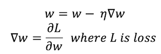
w represents the weight vector, η is the learning rate

Gradient Boosting Process:

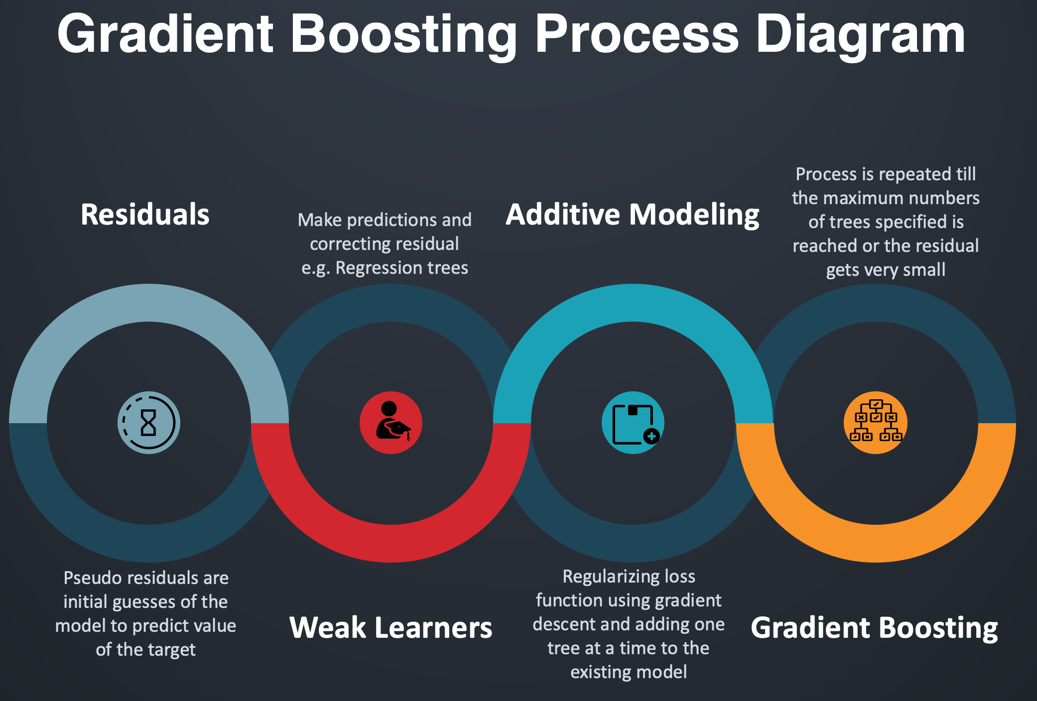
Process Flow of Gradient Boosting

Gradient boosting uses Additive Modeling in which a new decision tree is added one at a time to a model that minimizes the loss using gradient descent. Existing trees in the model remain untouched and thus slow down the rate of overfitting. The output of the new tree is combined with the output of existing trees until the loss is minimized below a threshold or specified limit of trees is reached.

Additive Modeling in mathematics is a breakdown of a function into the addition of N subfunctions. In statistical terms, it can be thought of as a regression model in which response y is the arithmetic sum of individual effects of predictor variables x.

XGBOOST In Action!

What makes XGBoost a go-to algorithm for winning Machine Learning and Kaggle competitions?

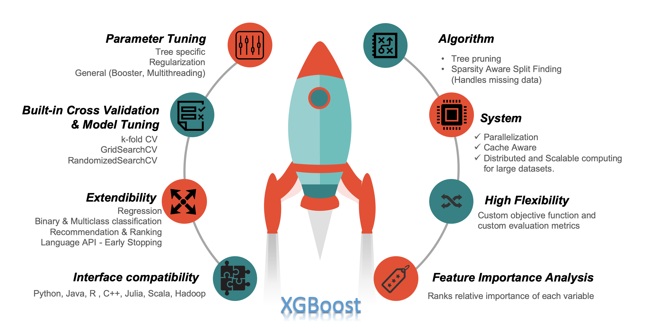
XGBoost Features

Isn’t it interesting to see a single tool to handle all our boosting problems! Here are the features with details and how they are incorporated in XGBoost to make it robust.

Algorithm Enhancements:

1. Tree Pruning — Pruning is a machine learning technique to reduce the size of regression trees by replacing nodes that don’t contribute to improving classification on leaves. The idea of pruning a regression tree is to prevent overfitting of the training data. The most efficient method to do pruning is Cost Complexity or Weakest Link Pruning, which internally uses mean square error, k-fold cross-validation and learning rate. XGBoost creates nodes (also called splits) up to max_depth specified and starts pruning from backward until the loss is below a threshold. Consider a split that has -3 loss and the subsequent node has +7 loss, XGBoost will not remove the split just by looking at one of the negative loss. It will compute the total loss (-3 + 7 = +4) and if it turns out to be positive it keeps both.
2. Sparsity Aware Split Finding — It is quite common that data that we gather has sparsity (a lot of missing or empty values) or becomes sparse after performing data engineering (feature encoding). To be aware of the sparsity pattern in data, a default direction is assigning it to each tree. XGBoost handles missing data by assigning them to default direction and finding the best imputation value so that it minimizes the training loss. Optimization here is to visit only missing values which make the algorithm run 50x faster than the naïve method.

System Enhancements:

1. Parallelization — Tree learning needs data in a sorted manner. To cut down the sorting costs, data is divided into compressed blocks (each column with corresponding feature value). XGBoost sorts each block parallelly using all available cores/threads of CPU. This optimization is valuable as a large number of nodes gets created frequently in a tree. In short, XGBoost parallelizes the sequential process of generating trees.
2. Cache Aware — By cache-aware optimization, we store gradient statistics (direction and value) for each split node in an internal buffer of each thread and perform accumulation in a mini-batch manner. This helps to reduce the time overhead of immediate read/write operations and also prevent cache miss. Cache awareness is achieved by choosing the optimal size of the block (generally 2^¹⁶).

Flexibility in XGBoost:

1. Customized Objective Function — An objective function intends to maximize or minimize something. In ML, we try to minimize the objective function which is a combination of the loss function and regularization term.

L(Φ) is objective function 

• reg: linear for regression
• reg: logistic, and binary: logistic for binary classification
• multi: softmax, and multi: softprob for multiclass classification

2. Customized Evaluation Metric — This is a metric used to monitor the model’s accuracy on validation data.

• rmse — Root mean squared error (Regression)
• mae — Mean absolute error (Regression)
• error — Binary classification error (Classification)
• logloss — Negative log-likelihood (Classification)
• auc — Area under the curve (Classification)

Cross-validation:

1. Built-in Cross-validation — Cross-validation is a statistical method to evaluate machine learning models on unseen data. It comes in handy when the dataset is limited and prevents overfitting by not taking an independent sample (holdout) from training data for validation. By reducing the size of training data, we are compromising with the features and patterns hidden in the data which can further induce errors in our model. This is similar to cross_val_score functionality provided by the sklearn library.

XGBoost uses built-in cross validation function cv():

xgb.cv() 

Want to get your feet wet? (It's coding time)

xxxxxxxxxx

## XGBOOST Cross Validation

import xgboost as xgb

import pandas as pd

from sklearn.datasets import load_boston

X, y = load_boston(return_X_y=True)

boston_dmatrix = xgb.DMatrix(data=X, label=y)

# 

reg_params = [1, 10, 100]

# params 

params = {"objective": "reg:squarederror", "max_depth": 3}

# Create an empty list for storing rmses as a function of ridge regression complexity

ridge_regression = []

# Iterate over reg_params

for reg in reg_params:

    # Update l2 strength

    params["lambda"] = reg

    # Pass this updated param dictionary into cv

    cv_results_rmse = xgb.cv(dtrain=boston_dmatrix, params=params, nfold=5, num_boost_round=5, metrics="rmse", as_pandas=True, seed=123)

    # Append best rmse (final round)

    ridge_regression.append(cv_results_rmse["test-rmse-mean"].tail(1).values[0])

# Look at best rmse per regularization param

print("Best RMSE as a function of ridge regression (L2 regularization):")

print(pd.DataFrame(list(zip(reg_params, ridge_regression)), columns=["l2", "rmse"]))

2. k-fold Cross-validation — In k-fold cross-validation, data is shuffled and divided into k equal sized subsamples. One of the k subsamples is used as a test/validation set and remaining (k -1) subsamples are put together to be used as training data. Then we fit a model using training data and evaluate using the test set. This process is repeated k times so that every data point stays in validation set exactly once. The k results from each model should be averaged to get the final estimation. The advantage of this method is that we significantly reduce bias and variance and also increase the robustness of the model.

k-fold Cross validation using sklearn in XGBoost :

from sklearn.model_selection import KFold, cross_val_score 

kfold = KFold(n_splits=1)

xgboost_score = cross_val_score(xg_cl, X, y, cv=kfold) 

Tuning Like a Pro! (Model Tuning)

Model tuning in XGBoost can be implemented by cross-validation strategies like GridSearchCV and RandomizedSearchCV.

1. Grid Search — We pass on a parameters’ dictionary to the function, it then compares the cross-validation score for each combination of parameters (many to many) in the dictionary and returns the set having the best parameters.

2. Random Search — Randomly draws a value during each iteration from the range of specified values for each hyperparameter searched over, and evaluates a model with those hyperparameters. After completing all iterations, it selects the hyperparameter configuration with the best score.

xxxxxxxxxx

## XGBOOST Model Tuning

import xgboost as xgb

import numpy as np

from sklearn.model_selection import GridSearchCV

from sklearn.model_selection import RandomizedSearchCV

from sklearn.datasets import load_boston

X, y = load_boston(return_X_y=True)

dmatrix = xgb.DMatrix(data=X, label=y)

# Grid Search Parameters

grid_search_params = {

    'colsample_bytree': [0.3, 0.7],

    'learning_rate': [0.01, 0.1, 0.2, 0.5],

    'n_estimators': [100],

    'subsample': [0.2, 0.5, 0.8],

    'max_depth': [2, 3, 5]

}

xg_grid_reg = xgb.XGBRegressor(objective= "reg:squarederror")

grid = GridSearchCV(estimator=xg_grid_reg, param_grid=grid_search_params, scoring='neg_mean_squared_error',

                    cv=4, verbose=1, iid=True)

grid.fit(X, y)

print("GridSearchCV")

print("Best parameters found: ", grid.best_params_)

print("Lowest RMSE found: ", np.sqrt(np.abs(grid.best_score_)))

# Random Search Parameters

params_random_search = {

    'learning_rate': np.arange(0.01, 1.01, 0.01),

    'n_estimators': [200],

    'max_depth': range(2, 12),

    'subsample': np.arange(0.02, 1.02, 0.02)

}

xg_random_reg = xgb.XGBRegressor(objective= "reg:squarederror")

randomized_mse = RandomizedSearchCV(param_distributions=params_random_search, estimator=xg_random_reg,

                                    scoring="neg_mean_squared_error", n_iter=5, cv=4, verbose=1, iid=True)

randomized_mse.fit(X, y)

print("Randomize Search Cross Validation")

print("Best parameters found: ", randomized_mse.best_params_)

print("Lowest RMSE found: ", np.sqrt(np.abs(randomized_mse.best_score_)))

output using grid search

output using random search

Total configurations in Grid Search → 2*4*1*3*3 = 72
Total configurations in Random Search → 100*1*10*50 = 50000

Extendibility:

1. Classification using XGBoost

xxxxxxxxxx

## XGBOOST Classification

import numpy as np

from numpy import loadtxt

import xgboost as xgb

from matplotlib import pyplot

from sklearn.model_selection import train_test_split

# load data

df = loadtxt('./dataset.csv', delimiter=",")

# Split data into X and y

X = df[:, 0:8]

y = df[:, 8]

# Spilt into train and test

X_train, X_test, y_train, y_test = train_test_split(X, y, test_size=0.2, random_state=123)

# XGB Classifier

xg_cl = xgb.XGBClassifier(objective='binary:logistic', n_estimators=100, seed=123)

eval_set = [(X_train, y_train), (X_test, y_test)]

# Fit the classifier to the training set

xg_cl.fit(X_train, y_train, eval_metric=["error"], eval_set=eval_set, verbose=True)

results = xg_cl.evals_result()

# Predict the labels of the test set: preds

predictions = xg_cl.predict(X_test)

# Compute the accuracy: accuracy

accuracy = float(np.sum(predictions == y_test))/y_test.shape[0]

print("accuracy: %f" % (accuracy*100))

# plot classification error

epochs = len(results['validation_0']['error'])

x_axis = range(0, epochs)

fig, ax = pyplot.subplots()

ax.plot(x_axis, results['validation_0']['error'], label='Train')

ax.plot(x_axis, results['validation_1']['error'], label='Test')

xgboost classification accuracy

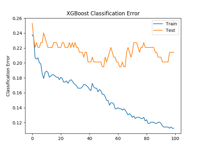
Classification Error

2. Regression using XGBoost:

2.1. Decision Tree Base Learning

xxxxxxxxxx

## XGBOOST Regression - Decision Tree Based

import xgboost as xgb

import pandas as pd

from sklearn.model_selection import train_test_split

from sklearn.metrics import explained_variance_score

# KC House Data

df = pd.read_csv('./kc_house_data.csv')

df_train = df[['bedrooms', 'bathrooms', 'sqft_living', 'floors', 'waterfront', 'view', 'grade', 'lat', 'yr_built', 'sqft_living15']]

X = df_train.values

y = df.price.values

X_train, X_test, y_train, y_test = train_test_split(X, y, test_size=0.2, random_state=123)

# Fitting XGB regressor model and default base learner is Decision Tree

xgb_reg = xgb.XGBRegressor(objective="reg:linear", n_estimators=75, subsample=0.75, max_depth=7)

xgb_reg.fit(X_train, y_train)

# Making Predictions

predictions = xgb_reg.predict(X_test)

# Variance_score

print((explained_variance_score(predictions, y_test)))

# To convert data table into a matrix

kc_dmatrix = xgb.DMatrix(data=X, label=y, feature_names=df_train)

# Create the parameter dictionary: params

params = {"objective": "reg:linear", "max_depth": 2}

# Train the model: xg_reg

xg_reg = xgb.train(params=params, dtrain=kc_dmatrix, num_boost_round=10)

# Plot the first tree as num_trees = 0 and features importance

xgb.plot_tree(xg_reg, num_trees=0)

xgb.plot_importance(xg_reg)

variance from xgboost regression with decision tree as base learner

Tree plots using decision tree (XGBRegressor)

2.2. Linear Base Learning

xxxxxxxxxx

## XGBOOST Regression Linear Base Learning

import numpy as np

import xgboost as xgb

from sklearn.datasets import load_boston

from sklearn.metrics import mean_squared_error

from sklearn.model_selection import train_test_split

# Linear Base Learner

X, y = load_boston(return_X_y=True)

# Train and test split

X_train, X_test, y_train, y_test = train_test_split(X, y, test_size=0.2, random_state=123)

# Convert the training and testing sets into DMatrixes

boston_train = xgb.DMatrix(data=X_train, label=y_train)

boston_test = xgb.DMatrix(data=X_test, label=y_test)

# Parameters with booster as gblinear for Linear base learner

params = {"booster": "gblinear", "objective": "reg:linear"}

# Train the model: xg_reg

xg_reg = xgb.train(params=params, dtrain=boston_train, num_boost_round=5)

# Making predictions

predictions = xg_reg.predict(boston_test)

# Computing RMSE

print("RMSE: %f" % (np.sqrt(mean_squared_error(y_test, predictions))))

rmse using xgboost regression with linear base learner 

Plot Importance Module:

XGBoost library provides a built-in function to plot features ordered by their importance. The function is plot_importance(model) and takes the trained model as its parameter. The function gives an informative bar chart representing the significance of each feature and names them according to their index in the dataset. The importance is calculated based on an importance_type variable which takes the parameters
weights (default) — tells the times a feature appears in a tree
gain — is the average training loss gained when using a feature
‘cover’ — which tells the coverage of splits, i.e. the number of times a feature is used weighted by the total training point that falls in that branch.

xgb.plot_importance(model)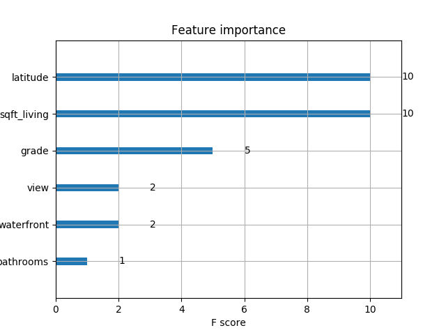 

Feature importance analysis on housing dataset 

Thanks for reading this article!

Co-authors — Rohan Harode, Akash Singh Kunwar

References

[1] https://arxiv.org/abs/1603.02754
[2] https://machinelearningmastery.com/gentle-introduction-xgboost-applied-machine-learning/
[3] https://explained.ai/gradient-boosting/index.html
[4] https://github.com/dmlc/xgboost
[5] https://towardsdatascience.com/ensemble-methods-bagging-boosting-and-stacking-c9214a10a205