Video Analysis to Detect Suspicious Activity Based on Deep Learning
Learn how to build on AI system that can classify a video into three classes: criminal or violent activity, potentially suspicious, or safe.
Join the DZone community and get the full member experience.
Join For FreeThis article explains one possible implementation of video classification. Our goal is to explain how we did it and the results we obtained so that you can learn from it.
Throughout this post, you will find a general description of the architecture of the solution, the methodology that we follow, the dataset we used, how we implemented it, and the results that we achieved.
Feel free to use this post as a starting point for developing your own video classifier.
The system described here is capable of classifying a video into three classes:
- Criminal or violent activity
- Potentially suspicious
- Safe
Our proposal to solve this problem is an architecture based on convolutional and recurrent neural networks.
Description of the Architecture of the Solution
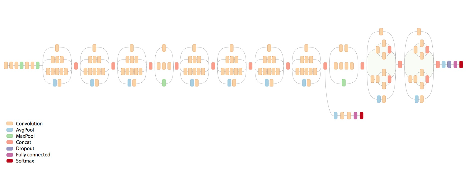
The first neural network is a convolutional neural network with the purpose of extracting high-level features of the images and reducing the complexity of the input. We will be using a pre-trained model called inception developed by Google. Inception-v3 is trained on the ImageNet Large Visual Recognition Challenge dataset. This is a standard task in computer vision, where models try to classify entire images into 1,000 classes like "zebra," "dalmatian," and "dishwasher."
We used this model to apply the technique of transfer learning. Modern object recognition models have millions of parameters and can take weeks to fully train. Transfer learning is a technique that optimizes a lot of this work by taking a fully trained model for a set of categories like ImageNet and retrains from the existing weights for new classes.
 Figure 1: Inception model
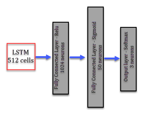
The second neural network used was a recurrent neural network, the purpose of this net is to make sense of the sequence of the actions portrayed. This network has an LSTM cell in the first layer, followed by two hidden layers (one with 1,024 neurons and relu activation and the other with 50 neurons with a sigmoid activation), and the output layer is a three-neuron layer with softmax activation, which gives us the final classification.
 Figure 2: Recurrent neural network
Methodology
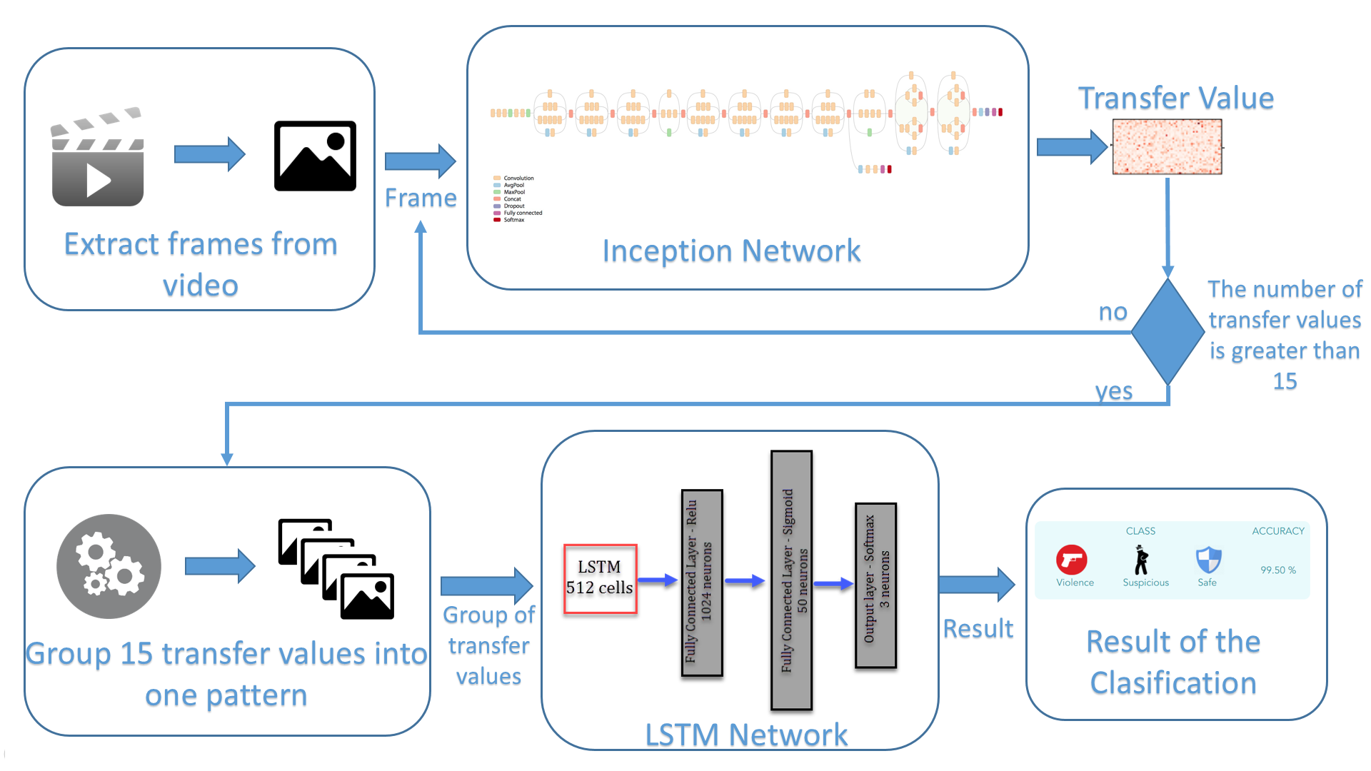
The first step is to extract the frames of the video. We extract a frame every 0.2 seconds and using this frame, we make a prediction using the inception model. Considering we are using the transfer learning technique, we are not going to extract the final classification of the inception model. Instead, we are extracting the result of the last pooling layer, which is a vector of 2,048 values (high-level feature map). Until now, we had a feature map of a single frame. Nevertheless, we want to give our system a sense of the sequence. To do so, we are not considering single frames to make our final prediction. We take a group of frames in order to classify not the frame but a segment of the video.
We consider that analyzing three seconds of video at a time is enough to make a good prediction of the activity that is happening at that moment. For this, we store fifteen feature maps generated by the inception model prediction, the equivalent of three seconds of video. Then, we concatenate this group of feature maps into one single pattern, which will be the input of our second neural network, the recurrent one, to obtain the final classification of our system.
 Figure 3: Video classification architecture
At the end, what we see on the screen is a classification of the video in real-time, where every three seconds, we see a classification of that part of the video — either safe, suspicious, or criminal activity.
Training Dataset
The dataset used for training the network is comprised of 150 minutes of screening divided into 38 videos. Most of these videos are recorded on security cameras of stores and warehouses. The result of taking a frame, each 0.2 seconds long, is having a dataset of 45,000 frames for training — the equivalent of 3000 segments of video, considering that a segment of a video represents three seconds of it (or 15 frames).
The whole dataset was labeled by us and divided into groups: 80% for training and 20% for testing.
As you can see, the final dataset is actually quite small. However, due to the transfer learning technique, we can get good results with fewer data. Of course, for the system to be more accurate, it’s better to have more data; that’s why we keep working on getting more and more data to improve our system.
 Figure 4: Data classes example
Implementation
The whole system was implemented with Python 3.5.
We use OpenCV for Python to segment the video in frames and resize them to 200x200px. Once we have all the frames, we make a prediction on the inception model using each of them. The result of each prediction is a “transfer value” representing the high-level feature map extracted from that specific frame. We save that in the transfer_values variable and its respective labels in the label_train variable.
Once we have these variables, we need to divide them into groups of 15 frames. We save the result in the joint_transfer variable.
frames_num=15
count = 0
joint_transfer=[]
for i in range(int(len(transfer_values)/frames_num)):
    inc = count+frames_num
    joint_transfer.append([transfer_values[count:inc],labels_train[count]])
    count =inc
Now that we have the transfer values and their labels, we can use this data to train our recurrent neural network. The implementation of this network is in Keras and the code for creating the model is as follows:
from keras.models import Sequential
from keras.layers import Dense, Activation
from keras.layers import LSTM
chunk_size = 2048
n_chunks = 15
rnn_size = 512
model = Sequential()
model.add(LSTM(rnn_size, input_shape=(n_chunks, chunk_size)))
model.add(Dense(1024))
model.add(Activation('relu'))
model.add(Dense(50))
model.add(Activation(sigmoid))
model.add(Dense(3))
model.add(Activation('softmax'))
model.compile(loss='mean_squared_error', optimizer='adam',metrics=['accuracy'])
The code above describes the construction of the model. The next step is about training it:
data =[]
target=[]
epoch = 1500
batchS = 100
for i in joint_transfer:
    data.append(i[0])
    target.append(np.array(i[1]))
model.fit(data, target, epochs=epoch, batch_size=batchS, verbose=1)
After we train the model, we need to save it as follows:
model.save("rnn.h5", overwrite=True)Now that the model is fully trained, we can start to classify videos.
Results and Other Possible Applications
After experimenting with different network architectures and tuning hyperparameters, the best result that we could achieve was 98% accuracy.
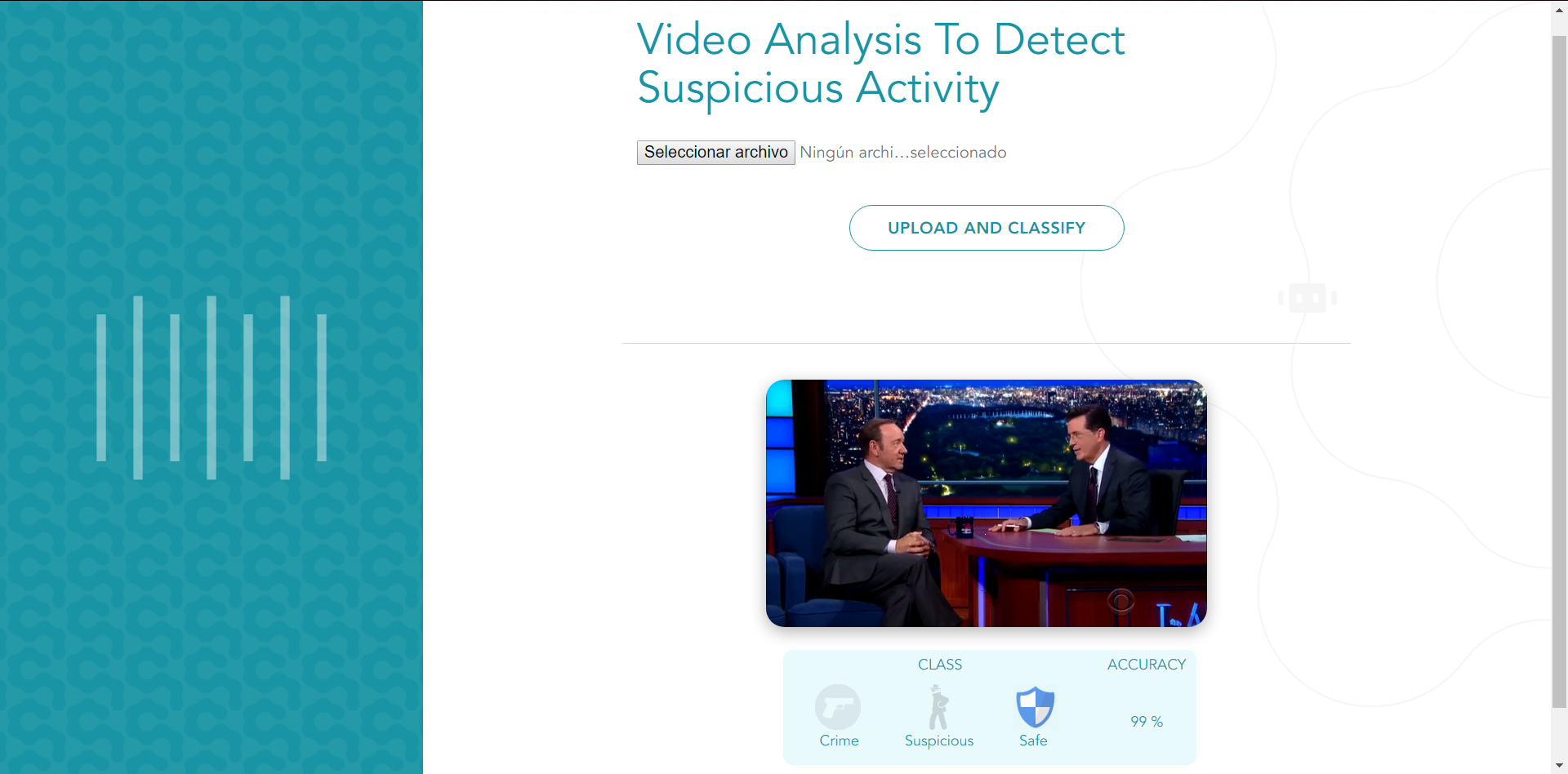
We designed the following front-end where you can upload a video and begin classifying it in real-time. You can see how the classes are constantly changing, as well as the respective accuracy for that class. These values constantly update every three seconds until the video is over.
 Figure 5: Front-end of the video classification
One of the things that we can do with this video classifier is to connect it to a security camera and keep analyzing the video in real-time, and the moment the system detects criminal or suspicious activity, it could activate an alarm or alert the police.
Furthermore, you can use a similar system trained with the appropriate data to detect different kinds of activities; for example, with a camera located in a school where your objective could be to detect bullying.
References
Opinions expressed by DZone contributors are their own.

Comments