Understanding Big O Notation in Python
Learning Big O notation is crucial because it helps us understand the current efficiency of our code and guides us in optimizing it further.
Join the DZone community and get the full member experience.
Join For FreeIn the world of programming, understanding the efficiency of your code is crucial. This is where concepts like time and space complexity come into play. In this blog post, we will explore these concepts in detail, focusing on how to calculate and interpret time complexity using Big O Notation. We will also look at practical examples in Python.
What Is Time Complexity?
Time complexity measures the efficiency of your code as the length of the input increases. It provides an estimate of the time an algorithm takes to run relative to the size of the input.
What Is Space Complexity?
Space complexity refers to the additional space taken by your code as the length of the input increases. It helps to understand the memory requirements of an algorithm.
Example: Time Complexity in Python
Let's say we have a list of 1000 numbers, and we need to print each number with an extra prefix or sentence before the elements:
numbers = [i for i in range(1000)]
for number in numbers:
    print(f"Number: {number}")
In this example, suppose, if printing each element takes 1 second, printing all 1000 elements would take 1000 seconds. If there is only 1 element, it takes 1 second. Therefore, the time taken is directly proportional to the size of the input.
Big O, Theta, and Omega Notations
- Big O Notation: Describes the worst-case scenario.
- Theta Notation: Describes the average-case scenario.
- Omega Notation: Describes the best-case scenario.
Big O Notation is the most widely used as it gives a clear understanding of the worst-case time and space complexity.
Practical Examples With Python Code
Let's dive into examples with code to understand these concepts better.
Example 1: Constant Time Complexity — O(1)
In the following function demo, the list is of size 3. We need to calculate the time complexity in terms of the list size. Here, we are printing the first element of the list. So, whether the list size is 3 or 3000, we are just printing the 0th element.
def demo(lst):
    print(lst[0])

demo([1, 2, 3])
The time complexity of this operation is O(1), which is constant time. As the size increases, the time remains constant.
Example 2: Linear Time Complexity — O(n)
In this code, the loop runs n times, making the time complexity O(n). This is known as linear complexity. As the input increases, the complexity increases linearly.
def print_elements(lst):
    for element in lst:
        print(element)

print_elements([1, 2, 3])
Example 3: Quadratic Time Complexity — O(n^2)
When there are two nested loops, the time complexity becomes quadratic, O(n^2). The outer loop runs n times and the inner loop runs m times.
def print_pairs(lst):
    for i in range(len(lst)):
        for j in range(len(lst)):
            print(lst[i], lst[j])

print_pairs([1, 2, 3])
Example 4: Cubic Time Complexity — O(n^3)
When there are three nested loops, the time complexity is cubic, O(n^3).
def print_triplets(lst):
    for i in range(len(lst)):
        for j in range(len(lst)):
            for k in range(len(lst)):
                print(lst[i], lst[j], lst[k])

print_triplets([1, 2, 3])
Example 5: Dominating Term
In a function with multiple complexities, we consider the term with the highest growth rate (dominating term).
def complex_function(lst):
    for i in range(len(lst)):  # O(n)
        print(lst[i])
    for i in range(len(lst)):  # O(n)
        for j in range(len(lst)):  # O(n^2)
            print(lst[i], lst[j])
    for i in range(len(lst)):  # O(n)
        for j in range(len(lst)):  # O(n)
            for k in range(len(lst)):  # O(n^3)
                print(lst[i], lst[j], lst[k])

complex_function([1, 2, 3])
The dominating term here is O(n^3).
Space Complexity in Python
Let's also understand space complexity with a practical example.
Example: Space Complexity
Consider the following function that creates a list of n elements.
def create_list(n):
    new_list = []
    for i in range(n):
        new_list.append(i)
    return new_list

create_list(1000)
In this example, the space complexity is O(n) because the space required to store the new_list grows linearly with the size of the input n. For every new element added to the list, we need additional space.
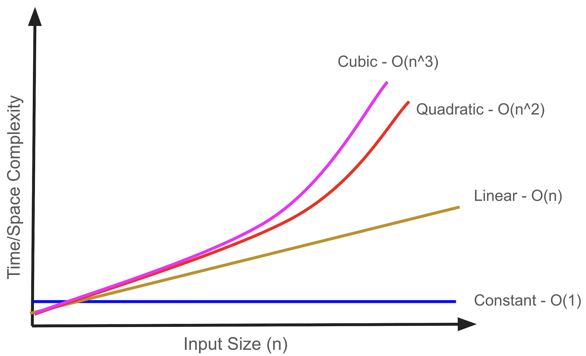
Complexity Graph
Understanding time and space complexity helps in optimizing code. With the following time/space complexity vs. input size graph, we can understand the different complexities. Constant time complexity is the best, and cubic time complexity is the worst. While optimizing code, the goal is to minimize complexity.

Opinions expressed by DZone contributors are their own.

Comments