Top 4 Regression Algorithms in Scikit-Learn
In AI, regression is a supervised machine learning algorithm that can predict continuous numeric values.
Join the DZone community and get the full member experience.
Join For FreeRegression is a robust statistical measurement for investigating the relationship between one or more independent (input features) variables and one dependent variable (output). In AI, regression is a supervised machine learning algorithm that can predict continuous numeric values. In simpler words, input features from the dataset are fed into the machine learning regression algorithm, which predicts the output values.
In this post, we’ll share a machine learning algorithms list of prominent regression techniques and discuss how supervised regression is implemented using the scikit-learn library.
1. Linear Regression
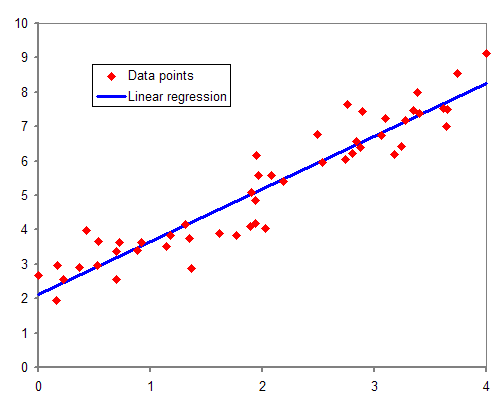
Linear regression is a machine learning algorithm that determines a linear relationship between one or more independent variables and a single dependent variable to predict the most suitable value of the dependent variable by estimating the coefficients of the linear equation.
The following straight-line equation defines a simple linear regression model that estimates the best fit linear line between a dependent (y) and an independent variable (x).
y=mx+c+eThe regression coefficient (m) denotes how much we expect y to change as x increases or decreases. The regression model finds the optimal values of intercept (c) and regression coefficient (m) such that the error (e) is minimized.
In machine learning, we use the ordinary least square method, a type of linear regression that can handle multiple input variables by minimizing the error between the actual value of y and the predicted value of y.
The following code snippet implements linear regression using the scikit-learn library:
# Import libraries
import numpy as np
from sklearn.linear_model import LinearRegression
# Prepare input data
# X represents independent variables
X = np.array([[1, 1], [1, 2], [1, 3], [2, 1], [2, 2], [2, 3]])
# Regression equation: y = 1 * x_0 + 2 * x_1 + 3
# y represents dependant variable
y = np.dot(X, np.array([1, 2])) + 3
# array([ 6,  8, 10,  7,  9, 11])
reg = LinearRegression().fit(X, y)
reg.score(X, y)
# Regression coefficients
reg.coef_
# array([1., 2.])
reg.intercept_
# 2.999999999999999
reg.predict(np.array([[4, 4]]))
# array([15.])
reg.predict(np.array([[6, 7]]))
array([23.])
2. Lasso Regression–Least Absolute Shrinkage and Selection Operator
Linear regression can overestimate regression coefficients, adding more complexity to the machine learning model. The model becomes unstable, large, and significantly sensitive to input variables.
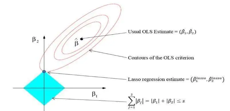
LASSO regression is an extension of linear regression that adds a penalty (L1) to the loss function during model training to restrict (or shrink) the values of the regression coefficients. This process is known as L1 regularization.
L1 regularization shrinks the values of regression coefficients for input features that do not make significant contributions to the prediction task. It brings the values of such coefficients down to zero and removes corresponding input variables from the regression equation, encouraging a simpler regression model.
The following code snippet shows how scikit-learn implements lasso regression in Python. In scikit-learn, the L1 penalty is controlled by changing the value of the alpha hyperparameter (tunable parameters in machine learning which can improve the model performance).
# Import library
from sklearn import linear_model
# Building lasso regression model with hyperparameter alpha = 0.1
clf = linear_model.Lasso(alpha=0.1)
# Prepare input data
X = np.array([[1, 1], [1, 2], [1, 3], [2, 1], [2, 2], [2, 3]])
y = [ 6,  8, 10,  7,  9, 11]
clf.fit([[0,0], [1, 1], [2, 2]], [0, 1, 2])
# Regression coefficients
clf.coef_
# array([0.6 , 1.85])
clf.intercept_
# 3.8999999999999995
clf.predict(np.array([[4, 4]]))
# array([13.7])
clf.predict(np.array([[6, 7]]))
# array([20.45])
3. The Ridge Regression Algorithm
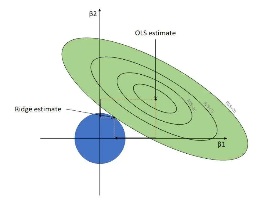
Ridge regression is another regularized machine learning algorithm that adds an L2 regularization penalty to the loss function during the model training phase. Like lasso, ridge regression also minimizes multicollinearity, which occurs when multiple independent variables show a high correlation with each other.
L2 regularization deals with multicollinearity by minimizing the effects of such independent variables, reducing the values of corresponding regression coefficients close to zero. Unlike L1 regularization, it prevents the complete removal of any variable.
The following code snippet implements ridge regression using the scikit-learn library. In scikit-learn, the L2 penalty is weighted by the alpha hyperparameter.
# Import library
from sklearn.linear_model import Ridge
# Building ridge regression model with hyperparameter alpha = 0.1
clf = Ridge(alpha=0.1)
# Prepare input data
X = np.array([[1, 1], [1, 2], [1, 3], [2, 1], [2, 2], [2, 3]])
y = [ 6,  8, 10,  7,  9, 11]
clf.fit(X, y)
clf.coef_
# array([0.9375, 1.95121951])
clf.intercept_
# 3.1913109756097553
clf.predict(np.array([[4, 4]]))
# array([14.74618902])
clf.predict(np.array([[6, 7]]))
# array([22.47484756])
4. The Elastic Net Regression Algorithm
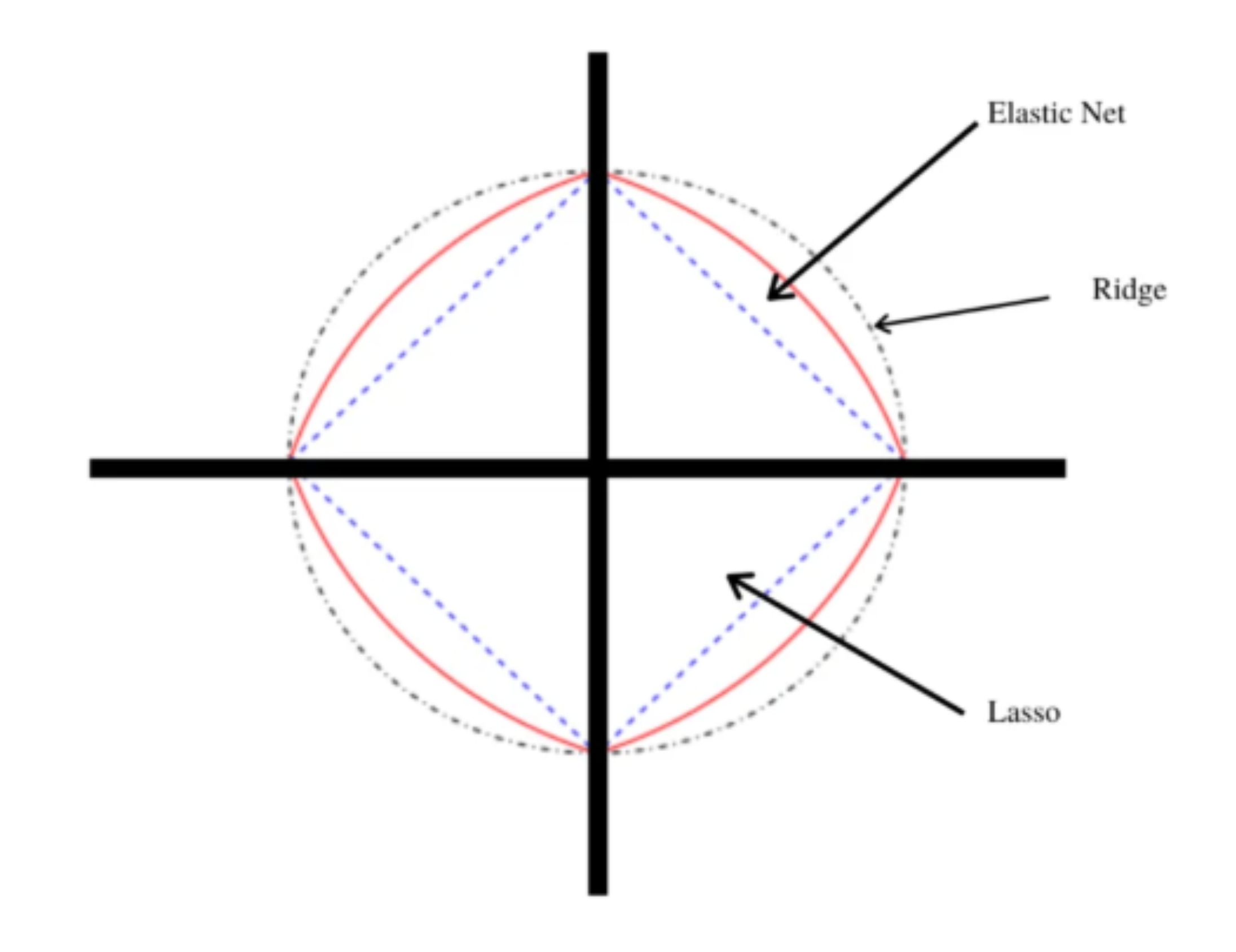
 Elastic net regression is a regularized linear regression algorithm that linearly combines both L1 and L2 penalties and adds them to the loss function during the training process. It balances lasso and ridge regression by assigning appropriate weight to each penalty, improving model performance.
Elastic net has two tunable hyperparameters, i.e., alpha and lambda. Alpha determines the percentage of weight given to each penalty, while lambda governs the percentage of the weighted sum of both liabilities that contribute toward model performance.
The following code snippet demonstrates elastic net regression using scikit-learn:
# Import library
from sklearn.linear_model import ElasticNet
# Building elastic net regression model with hyperparameter alpha = 0.1
regr = ElasticNet(alpha=0.1)
# Prepare input data
X = np.array([[1, 1], [1, 2], [1, 3], [2, 1], [2, 2], [2, 3]])
y = [ 6,  8, 10,  7,  9, 11]
regr.fit(X, y)
regr.coef_
# array([0.66666667, 1.79069767])
regr.intercept_)
# 3.9186046511627914
regr.predict([[4, 4]])
# array([13.74806202])
regr.predict([[0, 0]])
# array([20.45348837])
Regression Can Handle Linear Dependencies
Regression is a robust technique for predicting numerical values. The machine learning algorithms list provided above contains powerful regression algorithms that can conduct regression analysis and prediction for various machine learning tasks using the scikit-learn Python library.
However, regression is more suitable when the dataset contains linear relationships among dependent and independent features. To handle non-linear dependencies among data features, other regression algorithms, such as neural networks, are used as they can capture non-linearities using activation functions.
Published at DZone with permission of Stylianos Kampakis. See the original article here.
Opinions expressed by DZone contributors are their own.


Comments