Saving a Tree in Postgres Using LTREE

in one of my last posts , i showed you how to install and enable a postgres extension called ltree . ltree allows me to save, query on, and manipulate trees or hierarchical data structures using a relational database table. as we’ll see , using ltree i can count leaves, cut off branches, and climb up and down trees easily — all using sql right inside my application’s existing postgres database!

but trees are natural, haphazard, branching structures with countless leaves, while database tables are man-made rectangles full of numbers and text. how can i possibly save a beautiful tree structure into an ugly, boring database table?

path enumeration

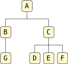
let’s return to the example tree from the first post in this series:

the ltree extension uses the path enumeration algorithm, which calls for each node in the tree to record the path from the root you would have to follow to reach that node.

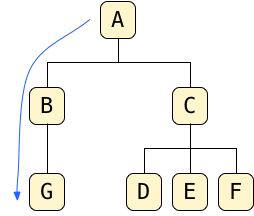
for example, to find g starting from a, the root, i would move down to b, and then down again to g:

so the path to g is:

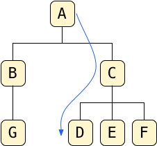
here’s another example:

this time i’ve traced a path from a to d, via c. so the path of d is:

saving tree paths using ltree

to use ltree, i need to create a column to hold these paths. for my example tree, i’ll use the same table i did before, but instead of the parent_id column, i’ll use a path column:

create table tree(
    id serial primary key,
    letter char,
    path ltree
);
create index tree_path_idx on tree using gist (path);

i chose the name path; i could have picked any name here. however, notice the path column uses a postgres data type called ltree — the ltree extension provides this special new type. and also notice i created a special gist index on the path column; more on this later!

next, i save the path of each tree node into the path column, encoded as a series of strings joined together by periods. for example, to save the path of g into my table, i use this insert statement:

and to save the path to node d, i write:

following this pattern, i can save my entire tree using these insert statements — one for each node in my tree:

insert into tree (letter, path) values ('a', 'a');
insert into tree (letter, path) values ('b', 'a.b');
insert into tree (letter, path) values ('c', 'a.c');
insert into tree (letter, path) values ('d', 'a.c.d');
insert into tree (letter, path) values ('e', 'a.c.e');
insert into tree (letter, path) values ('f', 'a.c.f');
insert into tree (letter, path) values ('g', 'a.b.g');

the root node, a, contains the simplest path a. its two child nodes, b and c, use paths a.b and a.c; the child nodes under c use paths a.c.d, a.c.e, etc. you get the idea.

the ancestor operator: @>

now for the fun part: ltree provides a series of new sql operators that allow me to query and manipulate tree data structures. the most powerful of these is @> , the “ancestor” operator. it tests whether one path is an ancestor of another.

returning to my question from the first post in this series , what if i needed to know how many children a had, recursively? that is, what if i needed to count its children, grandchildren, great-grandchildren, etc.? earlier we saw that using a parent_id column this would require an ever-increasing number of sql statements:

select count(*) from tree where parent_id = id;
select count(*) from tree where parent_id in (child ids);
select count(*) from tree where parent_id in (grandchild ids);
select count(*) from tree where parent_id in (great-grandchild ids);
select count(*) from tree where parent_id in (great_great-grandchild ids);

etc.

@> solves this problem for us. i can now recursively count the total number of nodes under any given parent like this:

select count(*) from tree where parent-path @> path;

in my example, this sql would return the number of nodes, recursively, under the root node a:

select count(*) from tree where 'a' @> path;
count 
-------
7
(1 row)

ltree counts the parent node itself, so the total count is 7, not 6. that is, a @> a evaluates to true . another example; this returns the count of tree nodes under and including c:

select count(*) from tree where ‘a.c' @> path;
count 
-------
4
(1 row)

or i could have written these predicates in the opposite order using <@ :

select count(*) from tree where path <@ 'a';
select count(*) from tree where path <@ 'a.c';

as you can see, the <@ and @> operators treat the path column, the column i defined with the ltree data type, as simple strings. but there’s some magic going on here: the path values are not simple strings. although i typed them in as strings, <@ and @> efficiently determine whether or not one path is an ancestor of another.

and the @> ancestor operator is just one way of using ltree columns; the ltree extension provides a long list of powerful operators and functions! for a complete list, see here .

in my next post , i’ll explore more of these functions and show you how to perform some tree operations that i’ve found useful.

maybe you’re not impressed

however, thinking about the path strings for a moment, it’s fairly obvious whether one path is an ancestor of another. for example, it’s clear that a and a.c are ancestors of a.c.d, while a.b is not. in fact, it looks like all the @> operator does it check whether the string on the left (the ancestor) is a prefix or leading substring inside the string on the right (the descendant).

in fact, you might not be very impressed by ltree, so far. the @> operator seems like a fancy way of performing a simple string operation. i could have written sql code to determine that a is an ancestor of a.c.d myself. i probably would have used one of postgres’s many string functions to achieve this, maybe something like this:

select count(*) from tree where strpos(path::varchar, 'a') = 1

postgres would calculate the answer for my seven-node example tree very quickly. but to calculate this count, internally postgres would have to iterate over all the records in my table (this is called a full table scan or sequence scan in db jargon) and calculate the strpos function on each row. if my tree had thousands or millions of rows, then this sql statement would take a long time to finish.

enabling the real magic: using a gist index with ltree

the power of the @> operator is that it allows postgres to search efficiently across an entire tree using an index. saying this in a more technical way: the @> operator integrates with postgres’s gist index api to find and match descendant nodes. to take advantage of this technology, be sure to create a gist index on your ltree column, for example like this:

create index tree_path_idx on tree using gist (path);

what is a “gist” index? how does it help ltree find and count tree nodes efficiently? read the last post in this series to find out. there i describe the generalized search index (gist) project, explore the computer science behind gist and look at how ltree uses gist to make fast tree operations inside of postgres possible.

what’s next?

but before we dive into ltree’s internal implementation, first we should see what else ltree can do. so far, i’ve shown you how to count descendant tree nodes. tomorrow, in my next post, manipulating trees using sql and the postgres ltree extension , i’ll show you how to use other ltree’s operators and functions to work with tree data.