Rolling Window Regression: A Simple Approach for Time Series Next Value Predictions

Given a time series, predicting the next value is a problem that fascinated programmers for a long time. Obviously, a key reason for this attention is stock markets, which promised untold riches if you can crack it. However, except for few (see A rare interview with the mathematician who cracked Wall Street), those riches have proved elusive.

Thanks to IoT (Internet of Things), time series analysis is poise to a come back into the limelight. IoT let us place ubiquitous sensors everywhere, collect data, and act on that data. IoT devices collect data through time and resulting data are almost always time series data.

The following are few use cases for time series prediction:

1. Power load prediction
2. Demand prediction for Retail Stores
3. Services (e.g. airline check-in counters, government offices) client prediction
4. Revenue forecasts
5. ICU care vital monitoring
6. Yield and crop prediction

Let’s explore the techniques available for time series forecasts.

The first question is that “isn’t it regression?”. It is close, but not the same as regression. In a time series, each value is affected by the values just preceding this value. For example, if there is a lot of traffic at 4.55 in a junction, chances are that there will be some traffic at 4.56 as well. This is called autocorrelation. If you are doing regression, you will only consider x(t) while due to auto correlation, x(t-1), x(t-2), … will also affect the outcome. So we can think about time series forecasts as regression that factor in autocorrelation as well.

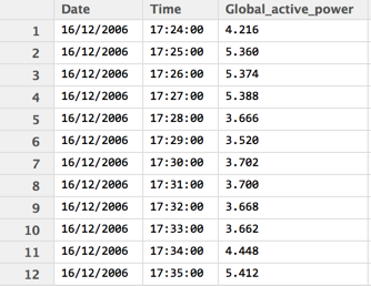
For this discussion, let’s consider “Individual household electric power consumption Data Set”, which is data collected from one household over four years in one-minute intervals. Let’s only consider three fields, and the data set will look like the following:

The first question to ask is how do we measure success? We do this via a loss function, where we try to minimize the loss function. There are several loss functions, and they are different pros and cons.

1. MAE ( Mean absolute error) — here all errors, big and small, are treated equally.
2. Root Mean Square Error (RMSE) — this penalizes large errors due to the squared term. For example, with errors [0.5, 0.5] and [0.1, 0.9], MSE for both will be 0.5 while RMSE is 0.5 and. 0.45.
3. MAPE ( Mean Absolute Percentage Error) — Since #1 and #2 depend on the value range of the target variable, they cannot be compared across data sets. In contrast, MAPE is a percentage, hence relative. It is like accuracy in a classification problem, where everyone knows 99% accuracy is pretty good.
4. RMSEP ( Root Mean Square Percentage Error) — This is a hybrid between #2 and #3.
5. Almost correct Predictions Error rate (AC_errorRate)—percentage of predictions that is within %p percentage of the true value

If we are trying to forecast the next value, we have several choices.

ARIMA Model

The gold standard for this kind of problems is ARIMA model. The core idea behind ARIMA is to break the time series into different components such as trend component, seasonality component etc and carefully estimate a model for each component. See Using R for Time Series Analysis for a good overview.

However, ARIMA has an unfortunate problem. It needs an expert (a good statistics degree or a grad student) to calibrate the model parameters. If you want to do multivariate ARIMA, that is to factor in multiple fields, then things get even harder.

However, R has a function called auto.arima, which estimates model parameters for you. I tried that out.

library("forecast")
....
x_train <- train data set
X-test <- test data set
..
powerTs <- ts(x_train, frequency=525600, start=c(2006,503604))
arimaModel <- auto.arima(powerTs)
powerforecast <- forecast.Arima(arimaModel, h=length(x_test))
accuracy(powerforecast)

You can find detail discussion on how to do ARIMA from the links given above. I only used 200k from the data set as our focus is mid-size data sets. It gave a MAPE of 19.5.

Temporal Features

The second approach is to come up with a list of features that captures the temporal aspects so that the auto correlation information is not lost. For example, Stock market technical analysis uses features built using moving averages. In the simple case, an analyst will track 7 days and 21 days moving averages and take decisions based on cross-over points between those values.

Following are some feature ideas

1. collection of moving averages/ medians(e.g. 7, 14, 30, 90 day)
2. Time since certain event
3. Time between two events
4. Mathematical measures such as Entropy, Z-scores etc.
5. X(t) raised to functions such as power(X(t),n), cos((X(t)/k)) etc

Common trick people use is to apply those features with techniques like Random Forest and Gradient Boosting, that can provide the relative feature importance. We can use that data to keep good features and drop ineffective features.

I will not dwell too much time on this topic. However, with some hard work, this method have shown to give very good results. For example, most competitions are won using this method (e.g. http://blog.kaggle.com/2016/02/03/rossmann-store-sales-winners-interview-2nd-place-nima-shahbazi /).

The down side, however, is crafting features is a black art. It takes lots of work and experience to craft the features.

Rolling Windows-based Regression

Now we got to the interesting part. It seems there is an another method that gives pretty good results without lots of hand holding.

Idea is to to predict X(t+1), next value in a time series, we feed not only X(t), but X(t-1), X(t-2) etc to the model. A similar idea has being discussed in Rolling Analysis of Time Series although it is used to solve a different problem.

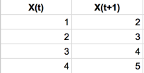
Let’s look at an example. Let’s say that we need to predict x(t+1) given X(t). Then the source and target variables will look like the following:

Data set would look like the following after transformed with rolling window of three:

Then, we will use above transformed data set with a well-known regression algorithm such as linear regression and Random Forest Regression. The expectation is that the regression algorithm will figure out the autocorrelation coefficients from X(t-2) to X(t).

For example, with the above data set, applying Linear regression on the transformed data set using a rolling window of 14 data points provided following results. Here AC_errorRate considers forecast to be correct if it is within 10% of the actual value.

LR AC_errorRate=44.0 RMSEP=29.4632 MAPE=13.3814 RMSE=0.261307

This is pretty interesting as this beats the auto ARIMA right way ( MAPE 0.19 vs 0.13 with rolling windows).

So we only tried Linear regression so far. Then I tried out several other methods, and results are given below.

Linear regression still does pretty well, however, it is weak on keeping the error rate within 10%. Deep learning is better on that aspect, however, took some serious tuning. Please note that tests are done with 200k data points as my main focus is on small data sets.

I got the best results from a Neural network with 2 hidden layers of size 20 units in each layer with zero dropout or regularization, activation function “relu”, and optimizer Adam(lr=0.001) running for 500 epochs. The network is implemented with Keras. While tuning, I found articles [1] and [2] pretty useful.

Then I tried out the same idea with few more datasets.

1. Milk production Data set ( small < 200 data points)
2. Bike sharing Data set (about 18,000 data points)
3. USD to Euro Exchange rate ( about 6500 data points)
4. Apple Stocks Prices (about 13000 data points)

Forecasts are done as univariate time series. That is we only consider time stamps and the value we are forecasting. Any missing value is imputed using padding (using most recent value). For all tests, we used a window of size 14 for as the rolling window.

The following tables shows the results. Here except for Auto.Arima, other methods using a rolling window based data set:

There is no clear winner. However, rolling window method we discussed coupled with a regression algorithm seems to work pretty well.

Conclusion

We discussed three methods: ARIMA, Using Features to represent time effects, and Rolling windows to do time series next value forecasts with medium size data sets.

Among the three, the third method provides good results comparable with auto ARIMA model although it needs minimal hand holding by the end user.

Hence we believe that “Rolling Window based Regression” is a useful addition to the forecaster’s bag of tricks!

However, this does not discredit ARIMA, as with expert tuning, it will do much better. At the same time, with hand-crafted features methods two and three will also do better.

One crucial consideration is picking the size of the window for rolling window method. Often we can get a good idea from the domain. Users can also do a parameter search on the window size.

The following are few things that need further exploration:

• Can we use RNN and CNN? I tried RNN, but could not get good results so far.
• It might be useful to feed other features such as time of day, day of the week, and also moving averages of different time windows.

Hope this was useful. If you enjoyed this post you might also like Stream Processing 101: From SQL to Streaming SQL and Patterns for Streaming Realtime Analytics. 

I write at https://medium.com/@srinathperera.