Introduction to Basic Statistics Measurements

This article is featured in the new DZone Guide to Big Data Get your free copy for more insightful articles, industry statistics, and more! 

Statistics consists of a body of methods for collecting and analyzing data (Agresti & Finlay, 1997). It is clear from the above definition that statistics is not only about the tabulation or visual representation of data. It is the science of deriving insights from data, and can be numerical (quantitative) or categorical (qualitative) in nature. Briefly, this science can be used to answer questions like:

• How much data is enough to perform a statistical analysis?

• What kind of data will require what sort of treatment?

Methods to draw the golden nuggets out of the data:

• Summarizing and exploring the data to understand the spread of the data, its central tendency, and its measure of association using various descriptive statistical methods.

• Drawing inferences from, forecasting, and generalizing the patterns displayed by the data to make some sort of conclusion.

• Furthermore, statistics is the art and science of dealing with events and phenomenon that are not certain in nature. They are used in every field of science.

The goal of statistics is to gain an understanding of data. Any data analysis should have the following steps:

1. Identify the research problem.

2. Define the sample and population.

3. Collect the data.

4. Perform descriptive and inferential analysis.

5. Use statistical research methods.

6. Solve the research problem.

Descriptive Statistics

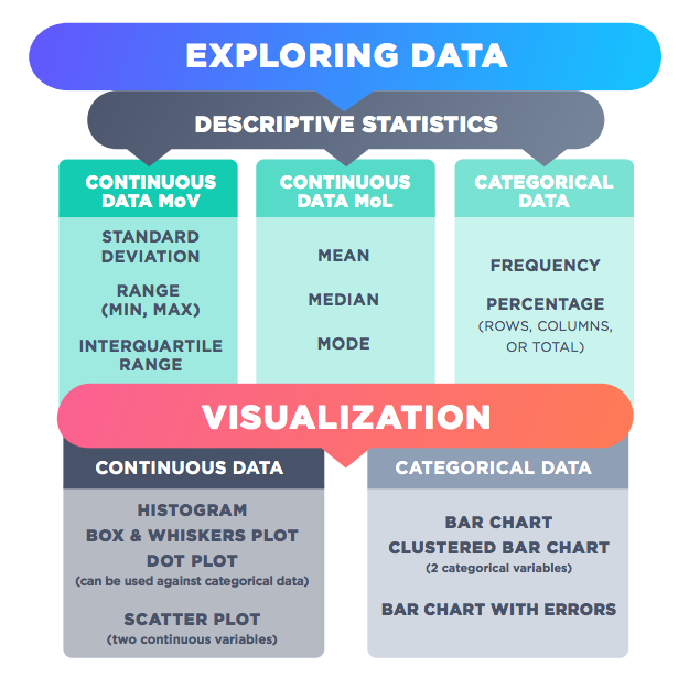
Descriptive statistics are summary statistics that quantitatively describe data using measures of central tendency and measures of variability or dispersion. The table below depicts the most commonly used descriptive statistics and visualization methods:

Descriptive statistics provide data summaries of the sample, along with the observations that have been made with regards to the sample data. Such summaries can be presented in the form of summary statistics (refer to the above visual for summary statistics types by data type) or easy-to-decipher graphs. It is worth mentioning here that descriptive statistics are mostly used to summarize values and may not be sufficient to make conclusions about the entire population or to infer or predict data patterns. Until now, we have just looked at the descriptive statistics that can be used to explore data by data type. This section of the article will help readers appreciate the nuances involved in using summary statistics.

Means and Averages

The term “mean” or “average” is one of the many summary statistics that can be used to describe the central tendency of the sample data. Computing this statistic is pretty straightforward: add all the values and divide the sum by the number of values to get the mean or average of the sample.

Example: The mean (or average) is (1+1+2+3+4)/5 = 2.2.

Median

The median is the value separating the higher half of a sample dataset from the lower half. The median can also be expressed as another way of finding the average of the sample data by sorting the number list from low to high and then finding the middle digit within the number list.

Example (one number in the middle):

Number list = 3, 2, 4, 1, 1.

Step 1: Sort the number list low to high = 1, 1, 2, 3, 4.

Step 2: Find the middle digit = 1, 1, 2, 3, 4.

Median = 2.

In the previous section, the mean/average for the same dataset was 2.2. However, the central tendency for the dataset using the median statistic is 2.

Example (two numbers in the middle):

With an even amount of numbers, things get little tricky. In this case, we have to identify the middle pair of numbers and then find the value that is halfway between them. This can be easily done by adding them together and dividing them by two.

Let’s look at an example where we have fourteen numbers, and we don’t have just one middle number; we have a pair of middle numbers.

Number list = 3, 13, 7, 5, 21, 23, 23, 40, 23, 14, 12, 56, 23, 29.

Step 1: Sort the number list from low to high = 3, 5, 7, 12, 13, 14,21, 23, 23, 23, 23, 29, 40, 56.

As stated previously, we don’t have just one middle number; we have a pair of middle numbers:

3, 5, 7, 12, 13, 14, 21, 23, 23, 23, 23, 29, 40, 56.

In the above example, the middle numbers are 21 and 23. To find the value halfway between them, add them together and divide by 2: 21 + 23 = 44 ÷ 2 = 22.

Median = 22.

(Note that 22 is not in the number list, but that is okay because half of the numbers in the list are less than 22 and half of the numbers are greater than 22.)

Variance/Delta and Standard Deviation

In my twenty years of experience, I have seen people use these two terms interchangeably when summarizing a dataset — which, in my opinion, is not only incorrect but also dangerous. You can call me a purist, but this is the distinction that we have to make to understand the difference between these two statistics.

Just to clear the air, I will take a step back and try to define these two terms in simple English and in statistical terms.

Variance can be defined as the average of the squared differences from the mean. Variance can be the difference between an expected result and an actual result, such as between a budget and an actual expenditure.

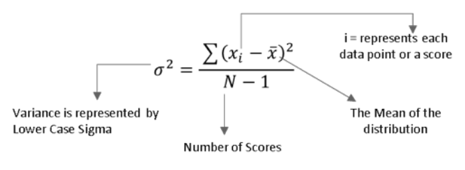
Variance Formula Demystified

I know that the above formula can be pretty daunting. Therefore, I will list out the steps to calculate the variance in an easy-to-understand manner:

1. Work out the mean.

2. Then, for each number, subtract the mean and square the results (squared difference).

3. Work out the averages of those squared values.

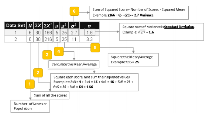
If you’re still unclear about all the math, let’s look at it visually to understand how to calculate the variance using a dataset.

Note: The square root of variance is called the standard deviation. Just like variance, standard deviation is used to describe the spread. Statistics like standard deviation can be more meaningful when expressed in the same units as the mean, whereas the variance is expressed in squared units.

Calculating Variance

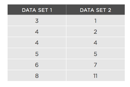
As an example, let’s look at two distributions and understand the step-by-step approach to calculating variance:

Here's how it works:

The above example helps us appreciate the intricacies involved in calculating the variance statistics, vis a vis stating that the variance or delta is the same thing.

Delta can be defined as a change or a difference in percentage, where we simply subtract the historic value from the most recent value and divide it with the recent value to get a Delta percent (some people call it variance percent, as well).

Example: (255 – 234)/234 = 9% (Delta %), and if we do not divide this by the recent number, we will get the pure delta = 21.

Standard Deviation Explained

Standard deviation is defined as “the deviation of the values or data from an average mean.”

Standard deviation helps us know how the values of a particular dataset are dispersed. A lower standard deviation concludes that the values are very close to their average, whereas higher values mean that the values are far from the mean value. Standard deviation values can never be negative.

Interpreting Ơ, standard deviation, using Chebyshev’s rule for any population:

• At least 75% of the observations will lie within 2Ơ of µ.

• At least 89% of the observations will lie within 3Ơ of µ.

• At least 100(1 – 1/m2)% of the observations will lie withinmxƠ of µ.

Things to remember about standard deviation:

• Use it when comparing unlike measures.

• It is the most common measure of spread.

• Standard deviation is the square root of the variance.

This article is featured in the new DZone Guide to Big Data Get your free copy for more insightful articles, industry statistics, and more!