From Dijkstra to A Star (A*), Part 1: The Dijkstra Algorithm

Finding a path from one node to another is a classic graph search problem that we can solve using multiple traversal algorithms like BFS or DFS. But, if we want to find the shortest path from one node to another, BFS or DFS traversals won’t help us too much, so we need to use other algorithms like Bellman-Ford, Floyd-Warshall or Dijkstra. In this article, I want to focus on the Dijkstra algorithm and see what we can do to improve it, to make it faster, thus, transforming it into an A star (A*) algorithm.

Finding the Shortest Path in a Positively Weighted Graph

In a positively weighted graph, we can calculate the path with the lowest cost from point A to point B, using the Dijkstra algorithm. If there are paths with negative costs, Dijkstra won’t work, so we would have to look to other methods, like Bellman-Ford or Floyd-Warshall algorithms.

The main idea of this algorithm is that starting from one node, the next node to visit is the one with the lowest cost over traversal from the source to it. So this looks almost like BFS, by having a queue with nodes, and, at each iteration, we pull an element from the queue and visit it. The difference between Dijkstra and BFS is that with BFS we have a simple FIFO queue, and the next node to visit is the first node that was added in the queue. But, using Dijkstra, we need to pull the node with the lowest cost so far.

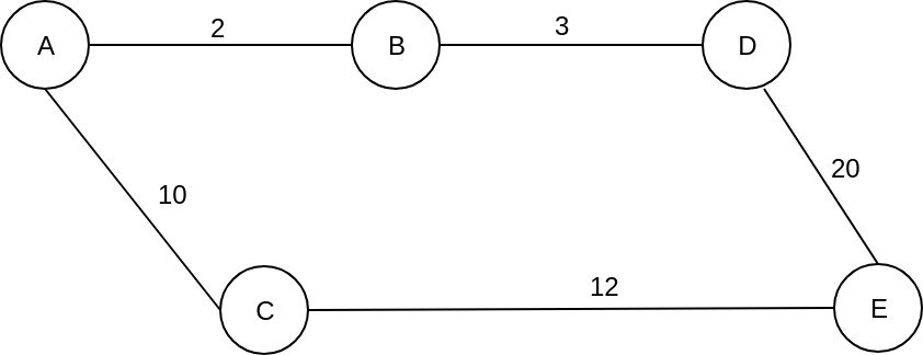
Let’s see a simple example:

We want to go from A to E using BFS, so, we'll use a simple FIFO queue. Starting from node A, we get the neighboring nodes, B and C, and we put them in the queue. Next, we pull from the queue the first element that has been added, node B, and we check the neighboring nodes, A and D. A was visited, so we ignore it, and we add node D to the queue. So the queue now contains nodes C and D.

We move forward and we get node C from the queue, check the neighboring nodes, A and E. We ignore A because we already visited it, and we see that we reached E and we stop. So we found a path, A -> C -> E, with a total cost of 22. Is this the path with the lowest cost? Well, no. Let’s change the algorithm to find the shortest path, by changing the way of retrieving the elements from the queue.

As a small observation, the classic BFS algorithm traverses all the graph, and it stops when the queue is empty. This is a slightly changed algorithm that's more greedy, where we stop when we find our destination.

So let's see what we get, if we pull from the queue the node with the lowest cost so far. Starting from A, we check the neighboring nodes, B and C, and we calculate the path cost from A to each of them. So we have a queue with:

Queue: {
  B, cost_so_far: 2
  C, cost_so_far: 10 
}

Now, using Dijkstra, we choose to visit the node with the lowest cost_so_far, which is B. We check the neighboring nodes, A and D, we see that node D doesn’t have any cost_so_far, and we calculate it. The cost_so_far for node D is the cost_so_far for B plus the cost between B and D, which is 3. So we have a total cost of 5. We put it in the queue and the queue will look like this:

Queue {
  C, cost_so_far: 10,
  D, cost_so_far: 5
}

Following the same process, we pull node D from the queue, because it has the lowest cost_so_far, despite the fact that C was added before. We check it, and we see that we reached E with a cost_so_far equal to 10 + 4 = 14. We add it in the queue, and, again, we choose the next node to visit from the queue. The queue will look like this:

Queue {
  E, cost_so_far: 14
  C, cost_so far: 10
}

We don’t stop here, but I will explain this a little later. But, for now, let’s continue the process. We look at the queue, and we pull the node with the lowest cost_so_far which is C. C has two neighbors, A which was visited before, and E with a cost_so_far equal to 14. Now, if we calculate the path cost to E, through C, we will have a cost_so_far equal to 22, which is greater than the current cost_so_far 14, so we don’t change it.

Moving forward, we will have a queue with one single node, E. We take it and we see that we reached our destination, so we stop. We now have the path with the lowest cost, from A to E, A -> B -> D -> E, with a total cost of 14. So, using BFS we found a path with the total cost of 22, but, using Dijkstra, we saw a better path with a lower cost of 14.

So, why didn’t we stop earlier when we first reached node E? Well, let’s change the edge cost between E and D to 20.

In this case, all the steps from A to D, will be the same. But, after we visit node D, the queue will look like this:

Queue {
  E, cost_so_far: 25
  C, cost_so far: 10
}

We take C, because it has the lowest cost_so_far, and we calculate the potential cost_so_far for E through C, which is 22, and we see that the new value is lower than the current cost_so_far, 25. So we update it and E will have a new cost_so_far equal to 22, through C. When we pull node E from the queue, we see that we reached our destination and we found the path with the lowest cost from A to E, which is A -> C -> E with a total cost of 22.

So, even if when we are visiting a node, we “see” our destination, and we calculate the cost_so_far for it, we don’t stop there, because there could be another path with a lower cost. So, every time we visit a node, we look to its neighbors and, even if we already calculated a cost_so_far when we previously visited another node, we check to see if we found a better path, by updating the cost_so_far if it is lower than the current one. That’s why the Dijkstra algorithm is able to find the path with the lowest cost.

Dijkstra Implementation Proposal

Let’s see how we can implement this. We will start with a node that has a name and an adjacency list for its neighbors. Beside those fields, we can also add a cost_so_far field, let's call it g_cost, and a parent. The searching algorithm will set these two fields and we will use them to find the path with the lowest cost from one node to another. We can initialize these fields by setting the g_cost to be infinite and the parent to be null. This could look like this:

static class Node{
  public final String name;
  public List<Edge> adjacency = new ArrayList<>();
  public Node parent;
  public double g_cost = Integer.MAX_VALUE;

  public Node(String name){
    this.name = name;
  }

  public void addNeighbour(Node neighbour, int cost) {
    Edge edge = new Edge(neighbour, cost);
    adjacency.add(edge);
  }

  public String toString(){
    return name;
  }
}

An edge has a cost and a target node.

static class Edge{
  public final double cost;
  public final Node target;

  public Edge(Node target, double cost){
    this.target = target;
    this.cost = cost;
  }
}

And now the algorithm. Like I said before, the main idea of this algorithm is that when starting from one node, the next node to be visited is the one with the lowest cost so far from the source to it. For this, we can use a Priority Queue, let’s called it a frontier, with nodes sorted by the g_cost. When we visit a node, if we find a better way for its neighbors, we just have to add them in the frontier and update the g_cost, and, since the frontier is a priority queue, it will maintain the nodes sorted by the g_cost  value. When we visit the destination, it means that we found the best path from source to destination and we stop.

This is the algorithm implementation:

public static void dijkstraSearch(Node source, Node destination) {
  source.g_cost = 0;

  PriorityQueue<Node> frontier = new PriorityQueue<>(new Comparator<Node>() {
    @Override
    public int compare(Node o1, Node o2) {
      return Double.compare(o1.g_cost, o2.g_cost);
    }
  });


  frontier.add(source);

  int numberOfSteps = 0;
  while (!frontier.isEmpty()) {
    numberOfSteps++;
    // get the node with minimum g_cost
    Node current = frontier.poll();

    System.out.println("Current node: " + current.name);

    // we have found the destination
    if (current.name.equals(destination.name)) {
      break;
    }

    // check all the neighbours
    for (Edge edge: current.adjacency) {

      Node neigh = edge.target;
      double cost = edge.cost;

      double newCost = current.g_cost + cost;

      if (newCost < neigh.g_cost) {
        neigh.parent = current;
        neigh.g_cost = newCost;

        // reset frontier order
        if (frontier.contains(neigh)) {
          frontier.remove(neigh);
        }

        frontier.add(neigh);
      }
    }
  }

  System.out.println("Number of steps: " + numberOfSteps);
}

Again, as I said before about the BFS implementation, this is a slightly modified version of the Dijkstra algorithm, called Uniform Cost Search, where we stop when we find the destination. The classic Dijkstra algorithm continues to visit all the nodes until the queue is empty, finding the minimum path cost from the start node to every other node.

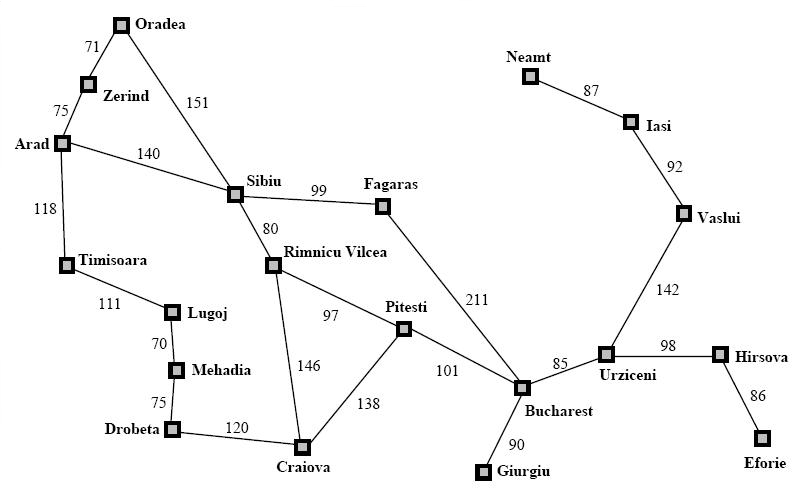
Let’s see how this works on a real map. Below is a map of Romania. Let's say that we want to drive from Arad to Bucharest on the shortest path.

We can see that there are multiple routes that we can take. We can go from Arad to Timisoara, then Lugoj, and so on, or we can choose Sibiu then Fagaras and go straight to Bucharest. But we don’t know which path has the lowest cost. So, this is a good candidate for the Dijkstra algorithm. Running our implementation on the Romanian map will get this:

Total Cost: 418.0
Path: [Arad, Sibiu, Rimnicu Vilcea, Pitesti, Bucharest]

That’s the path with the lowest cost (trust me, I am actually from Romania and I can assure you that this is the shortest way). So, using the Dijkstra algorithm we were able to find the path with the lowest cost, but let’s see how many steps were necessary to find this by printing the nodes when visiting them:

Current node: Arad
Current node: Zerind
Current node: Timisoara
Current node: Sibiu
Current node: Oradea
Current node: Rimnicu Vilcea
Current node: Lugoj
Current node: Fagaras
Current node: Mehadia
Current node: Pitesti
Current node: Craiova
Current node: Drobeta
Current node: Bucharest
Number of steps: 13

So we need to visit 13 nodes to find the best path. As you can see, from Arad we didn’t go straight to Sibiu, we got there via Zerind, then Timisoara, and then Sibiu. And, even after that, we didn’t go to Rimnicu Valcea, but to Oradea, because that was the node with the lowest cost so far. That’s how this algorithm works. Thirteen nodes to visit in order to find our path and many of those nodes aren’t on the path with the lowest cost anyway. But we didn’t know that and we had to visit them to find out.

That's all for Part 1! Come abck on Monday when we'll cover how to solve this problem using the A Star [A(*)] algorithm.