Building Predictive Analytics for Loan Approvals

In this short article, we'll explore loan approvals using a variety of tools and techniques. We'll begin by analyzing loan data and applying Logistic Regression to predict loan outcomes. Building on this, we'll integrate BERT for Natural Language Processing to enhance prediction accuracy. To interpret the predictions, we'll use SHAP and LIME explanation frameworks, providing insights into feature importance and model behavior. Finally, we'll explore the potential of Natural Language Processing through LangChain to automate loan predictions, using the power of conversational AI.

The notebook file used in this article is available on GitHub.

Introduction

In this article, we'll explore various techniques for loan approvals, using models like Logistic Regression and BERT, and applying SHAP and LIME for model interpretation. We'll also investigate the potential of using LangChain for automating loan predictions with conversational AI.

Create a SingleStore Cloud Account

A previous article showed the steps to create a free SingleStore Cloud account. We'll use the Free Shared Tier and take the default names for the Workspace and Database.

Import the Notebook

We'll download the notebook from GitHub (linked earlier).

From the left navigation pane in the SingleStore Cloud portal, we'll select DEVELOP > Data Studio.

In the top right of the web page, we'll select New Notebook > Import From File. We'll use the wizard to locate and import the notebook we downloaded from GitHub.

Run the Notebook

After checking that we are connected to our SingleStore workspace, we'll run the cells one by one.

We'll begin by installing the necessary libraries and importing dependencies, followed by loading the loan data from a CSV file containing nearly 600 rows. Since some rows have missing data, we'll drop the incomplete ones for the initial analysis, reducing the dataset to around 500 rows.

Next, we'll further prepare the data and separate the features and target variables.

Visualizations can provide great insights into data, and we'll begin by creating a heatmap that shows the correlation between numeric-only features, as shown in Figure 1.

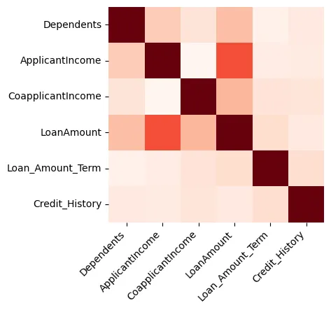
Figure 1: Heatmap

We can see that the Loan Amount and the Applicant Income are strongly related.

If we plot the Loan Amount against Applicant Income, we can see that most of the data points are towards the bottom left of the scatter plot, as shown in Figure 2.

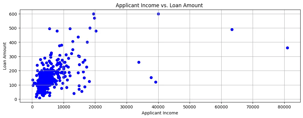
Figure 2: Scatter Plot

So, incomes are generally quite low and loan applications are also for fairly small amounts.

We can also create a pair plot for the Loan Amount, Applicant Income, and Co-applicant Income, as shown in Figure 3.

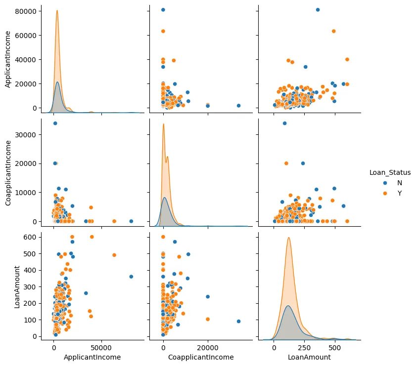
Figure 3: Pair Plot

In most cases, we can see that the data points tend to cluster together and there are generally few outliers.

We'll now perform some feature engineering. We'll identify the categorical values and convert these to numerical values and also use one-hot encoding where required.

Next, we'll create a model using Logistic Regression as there are only two possible outcomes: either a loan application is approved or it is denied.

If we visualize the feature importance, we can make some interesting observations, as shown in Figure 4.

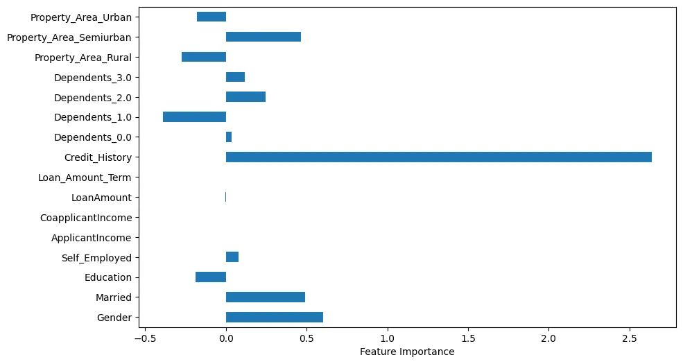
Figure 4: Feature Importance

For example, we can see that Credit History is obviously very important. However, Marital Status and Gender are also important.

We'll now make predictions using one test sample.

We'll generate a loan application summary using Bidirectional Encoder Representations from Transformers (BERT) with the test sample. Example output:

BERT-Generated Loan Application Summary

applicant : mr blobby income : $ 7787. 0 credit history : 1. 0 loan amount : $ 240. 0 property area : urban area

Model Prediction ('Y' = Approved, 'N' = Denied): Y
Loan Approval Decision: Approved

Using the BERT-generated summary, we'll create a word cloud as shown in Figure 5.

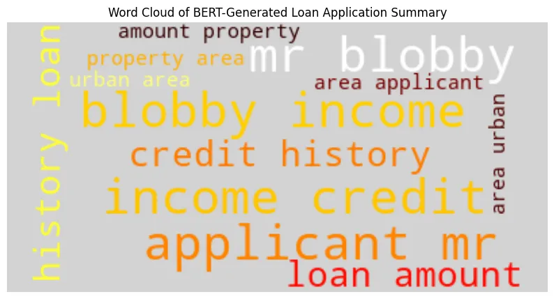
We can see that the applicant's name, income, and credit history are larger and more prominent.

Another way we can analyze the data for our test sample is by using SHapley Additive exPlanations (SHAP). In Figure 6 we can visually see features that are important.

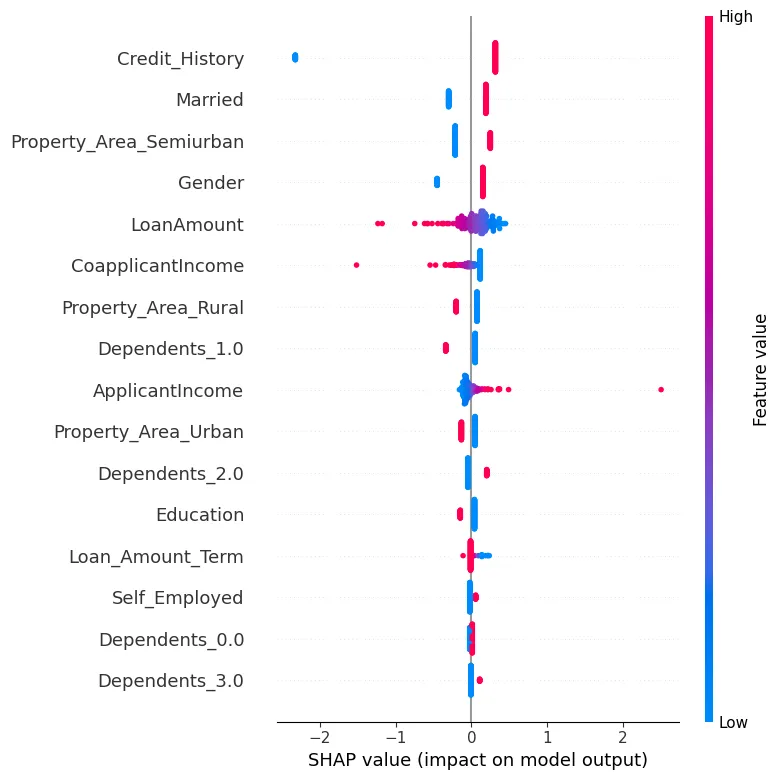
Figure 6: SHAP

A SHAP force plot is another way we could analyze the data, as shown in Figure 7.

Figure 7: Force Plot

We can see how each feature contributes to a particular prediction for our test sample by showing the SHAP values in a visual way.

Another very useful library is Local Interpretable Model-Agnostic Explanations (LIME). The results for this can be generated in the accompanying notebook to this article.

Next, we'll create a Confusion Matrix (Figure 8) for our Logistic Regression model and generate a classification report.

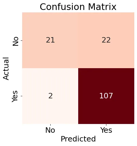
Figure 8: Confusion Matrix

The results shown in Figure 8 are a little mixed, but the classification report contains some good results:

Accuracy: 0.84
Precision: 0.83
Recall: 0.98
F1-score: 0.90
Classification Report:
              precision    recall  f1-score   support

           N       0.91      0.49      0.64        43
           Y       0.83      0.98      0.90       109

    accuracy                           0.84       152
   macro avg       0.87      0.74      0.77       152
weighted avg       0.85      0.84      0.82       152

Next, let's use LangChain and an LLM and see if we can also make loan predictions.

Once we have set up and configured LangChain, we'll test it with two examples, but restrict access to the quantity of data so that we don't exceed token and rate limits. Here is the first example:

query1 = (
"""
    Build a loan approval model.
    Limit your access to 10 rows of the table.
    Use your model to determine if the following loan would be approved:
    Gender: Male
    ApplicantIncome: 7787.0
    Credit_History: 1
    LoanAmount: 240.0
    Property_Area_Urban: 1
    Limit your reply to either 'Approved' or 'Denied'.
"""
)

result1 = run_agent_query(query1, agent_executor, error_string)
print(result1)

In this case, the application was approved in the original dataset.

Here is the second example:

query2 = (
"""
    Build a loan approval model.
    Limit your access to 10 rows of the table.
    Use your model to determine if the following loan would be approved:
    Gender: Female
    ApplicantIncome: 5000.0
    Credit_History: 0
    LoanAmount: 103.0
    Property_Area_Semiurban: 1
    Limit your reply to either 'Approved' or 'Denied'.
"""
)

result2 = run_agent_query(query2, agent_executor, error_string)
print(result2)

In this case, the application was denied in the original dataset.

Running these queries, we may get inconsistent results. This may be due to restricting the quantity of data that can be used. We can also use verbose mode in LangChain to see the steps being used to build a loan approval model, but there is insufficient information at this initial level about the detailed steps to create that model.

More work is needed with conversational AI, as many countries have fair lending rules and we'd need a detailed explanation about why the AI approved or denied a particular loan application.

Summary

Today, many powerful tools and techniques enhance Machine Learning (ML) for deeper insights into data and loan prediction models. AI, through Large Language Models (LLMs) and modern frameworks, offers great potential to augment or even replace traditional ML approaches. However, for greater confidence in AI's recommendations and to comply with legal and fair lending requirements in many countries, it's crucial to understand the AI's reasoning and decision-making process.