Bill of Materials in Neo4j

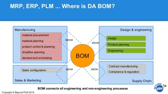
Where is da BOM? the above question asks, and the obvious answer is right in the middle of your organization, nestled between manufacturing, design, sales, and supply chain. But I have a better answer. Your Bill of Materials should be in Neo4j. Today, I'll show you why.

Let's start with a simple example first by creating a BOM in Neo4j.

CREATE (a1:Asset {id:'a1'})
CREATE (p1:Part {id:'p1'})
CREATE (p2:Part {id:'p2'})
CREATE (p3:Part {id:'p3'})
CREATE (p4:Part {id:'p4'})
CREATE (p5:Part {id:'p5'})
CREATE (a1)<-[:BELONGS_TO]-(p1)
CREATE (p1)<-[:BELONGS_TO]-(p2)
CREATE (p1)<-[:BELONGS_TO]-(p4)
CREATE (p2)<-[:BELONGS_TO]-(p3)
CREATE (p4)<-[:BELONGS_TO]-(p5)

After we run that command, our graph looks like this:

If we want to know all the parts that are needed to produce Asset 1, we could run this query:

MATCH (n:Asset {id:'a1'})<-[:BELONGS_TO*]-(p)
RETURN DISTINCT p

The query finds the asset with an ID of a1 and then traverses all the incoming BELONGS_TO  relationships all the way to the end. That's what the little * at the end of the relationship type in our query means. Knowing that some parts may belong in multiple downlines, we use DISTINCT  to only see them once in our result.

So that's pretty simple so far. Let's delete all that (for those following along in front of Neo4j run MATCH (n) DETACH DELETE n), and create a bigger graph. You can see the whole thing if you follow this link, but for now, I'll just show you want it looks like:

We have 3 Families of products with 7 Assets, and 15 Parts between them. Part 14 is common across them. So let's start asking a few questions.

Take a look at Part 14. What Assets require Part 14 in order to be built?

MATCH path=(p14:Part {id:'p14'})-[:BELONGS_TO*]->(a:Asset)
RETURN DISTINCT a

It is in the paths of Assets 1, 3, 4, 5, 6, and 7. But what is the lowest level this part is used at? Assuming Asset is level 0, then this query returns the longest path, and shows p14 has a depth of 5

MATCH path=(p14:Part {id:'p14'})-[:BELONGS_TO*]->(a:Asset)
WITH path, LENGTH(path) AS depth
RETURN path, depth
ORDER BY depth DESC
LIMIT 1

If we wanted to set the lowest depth, we can modify the query this way:

MATCH path=(p14:Part {id:'p14'})-[:BELONGS_TO*]->(a:Asset)
WITH p14, path, LENGTH(path) AS depth
ORDER BY depth DESC
LIMIT 1
SET p14.depth = depth

Can we compare two bills of material (two Assets) and find out common parts are used in both and components unique to each? Let's try Asset 3 and Asset 5. Here is the query:

MATCH path_a3 = (a3:Asset {id:'a3'})<-[:BELONGS_TO*]-(p3), 
      path_a5 = (a5:Asset {id:'a5'})<-[:BELONGS_TO*]-(p5)
WITH COLLECT(DISTINCT p3) AS a3_parts, COLLECT(DISTINCT p5) AS a5_parts
RETURN filter(x IN a3_parts WHERE NOT(x IN a5_parts)) AS unique_a3, 
       filter(x IN a5_parts WHERE NOT(x IN a3_parts)) AS unique_a5, 
       filter(x IN a3_parts WHERE (x IN a5_parts)) AS common

We start from each asset, traverse all the BELONGS_TO paths, and collect the distinct parts we find. Then we use the FILTER function to get the unique parts and the common parts of the two assets. Pretty simple, right? Let's up the difficulty a tiny bit by comparing the BOMs of two families of assets. Again to identify common and unique items.

MATCH path_f1 = (f1:Family {id:'f1'})<-[:BELONGS_TO]-(:Asset)<-[:BELONGS_TO*]-(p1), 
      path_f3 = (f3:Family {id:'f3'})<-[:BELONGS_TO]-(:Asset)<-[:BELONGS_TO*]-(p3)
WITH COLLECT(DISTINCT p1) AS f1_parts, 
     COLLECT(DISTINCT p3) AS f3_parts
RETURN filter(x IN f1_parts WHERE NOT(x IN f3_parts)) AS unique_f1, 
       filter(x IN f3_parts WHERE NOT(x IN f1_parts)) AS unique_f3, 
       filter(x IN f1_parts WHERE (x IN f3_parts)) AS common

Those are simplified examples, of course; how would you introduce the number of parts required for our model? Let's try an example:

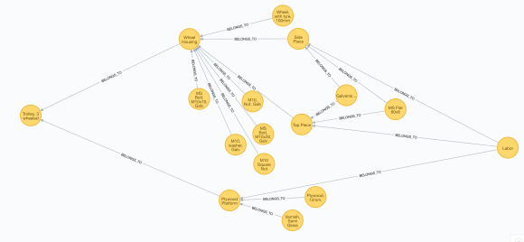
Here we are modeling a sample trolley. The nodes and relationships would look like this:

CREATE (a1:Part {id:"120-001", desc:"Trolley, 3 wheeled"})
CREATE (p1:Part {id:"110-001", desc:"Wheel Housing"})
CREATE (p2:Part {id:"100-001", cost: 5.30, desc:"MS Bolt, M10x70, Galv"})
...
CREATE (a1)<-[:BELONGS_TO {qty:3.0, unit:"EA"}]-(p1)
CREATE (p1)<-[:BELONGS_TO {qty:1.0, unit:"EA"}]-(p2)
CREATE (p1)<-[:BELONGS_TO {qty:2.0, unit:"EA"}]-(p3)

We retain the part ID, description, and, in some cases, the cost of the parts in the nodes and the quantity required as well as the measurement unit in the relationships. The full command to generate the graph is on the second file of this link and our graph looks like:

Now, how much does it cost to build the trolley? It should be as simple as:

MATCH (t:Part {id:"120-001"})<-[r:BELONGS_TO]-(p:Part)
RETURN SUM(r.qty * p.cost)

But it isn't because we haven't aggregated our individual parts up along the way. We can see the "Wheel Housing" node has no cost property. So how do we fix this? Well, we have two options. One we can dynamically calculate the price, but we will be doing that every time and that seems wasteful. The other option is to pre-calculate those combined costs and save them in the part nodes. There is probably a better way to do this, if you know it, add it in the comments.

One way is to find all the nodes in the path that do not have a cost property and that are the last nodes along the path not to have a cost property. We need this to be true in order to be able to set their cost. The query below does that, we will run it until we get "no changes, no records" returned meaning that all part nodes now have a cost. The first time it is run, it calculates the part_cost for the "Top Piece," "Side Piece," and "Plywood Platform." The second time it calculates the part_cost for the "Wheel Housing" which required "Top Piece" and "Side Piece" to be calculated first, and then the third time it calculates the price for the Trolley. The fourth time it does nothing.

MATCH path = (t:Part {id:"120-001"})<-[:BELONGS_TO*0..]-(:Part)
WHERE last(nodes(path)).cost is null
WITH t, last(nodes(path)) AS missing_cost
WITH t, missing_cost, SIZE(COLLECT(missing_cost)) AS need_cost
MATCH path = (missing_cost)<-[:BELONGS_TO*0..]-(p:Part)
WITH t, missing_cost, need_cost, COLLECT(DISTINCT p) AS parts
WHERE SINGLE(x IN parts WHERE COALESCE(x.cost, x.part_cost) IS NULL)
MATCH (missing_cost)<-[r:BELONGS_TO]-(p:Part)
WITH missing_cost, SUM(r.qty * COALESCE(p.cost, p.part_cost)) AS part_cost
WHERE NOT EXISTS(missing_cost.part_cost)
SET missing_cost.part_cost = part_cost

Now, we can check our price and...

MATCH (t:Part {id:"120-001"}) RETURN t.part_cost

246.965 — as expected.

Pretty cool, right? And all except that last query were pretty simple to write. Now, a real BOM system will have versions, it will have replacement parts, and it will have all kinds of complications, but I promise you — it's nothing Neo4j can't handle.

If you haven't yet, also take a look at this blog post from my colleague Rik Van Bruggen on Using Neo4j to Manage and Calculate Hierarchies. If you are interested in seeing the bigger picture, this blog post shows you how the German toy manufacturer Schleich uses a graph data model to track all the elements related to toy production.