A Review of Graph Databases

There are many ideas and considerations behind graph databases. This includes their use cases, advantages, and the trends behind this database model. There are also several real-world examples to dissect.

A Social Network Scenario

In a social network scenario, a user can post, share someone else’s post, comment on other people’s or advertiser posts, follow each other, and so on. For such a data-driven social media company, it is essential to pursue a basic CRUD (Create, Read, Update, Delete) operation to add more people, add new messages to the current database or find associated information. This helps the company figure out a certain user’s profile. For example, it might find that user Jeff has many posts relating to AI and music. Thus we may conclude him being a programmer, and so on.

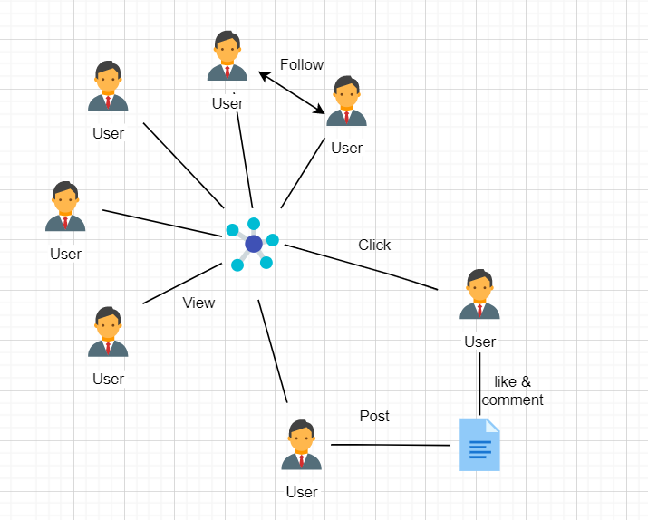
Sometimes requirements for one analysis can be extremely tricky. For example, you might have a query for Find all posts from users and count the number of posts up to 3 levels down [1]. Such an analytic problem is not purposely designed to create obstructions for data engineers, Indeed, these things are quite common in the current era of distributed computing.

Traditional Ways to Solve the Question

Data Model Schemes and Traditional Queries

The traditional way to solve this query need is to build a relational data model for every user and store those relations in several tables. This is commonly done in a Relational database such as MySQL.

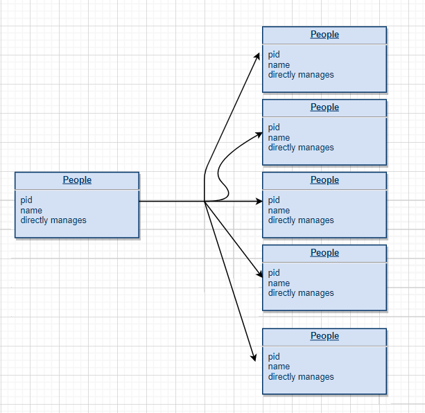
This is a basic relational schema.

If we want to implement a query as noted, it is inevitable that there will be a huge amount of JOIN and the length of query can be extremely long. [1]

(SELECT T.directReportees AS directReportees, sum(T.count) AS count

FROM (

SELECT manager.pid AS directReportees, 0 AS count

    FROM person_reportee manager

    WHERE manager.pid = (SELECT id FROM person WHERE name = "fName lName")

UNION

    SELECT manager.pid AS directReportees, count(manager.directly_manages) AS count

FROM person_reportee manager

WHERE manager.pid = (SELECT id FROM person WHERE name = "fName lName")

GROUP BY directReportees

UNION

SELECT manager.pid AS directReportees, count(reportee.directly_manages) AS count

FROM person_reportee manager

JOIN person_reportee reportee

ON manager.directly_manages = reportee.pid

WHERE manager.pid = (SELECT id FROM person WHERE name = "fName lName")

GROUP BY directReportees

UNION

SELECT manager.pid AS directReportees, count(L2Reportees.directly_manages) AS count

FROM person_reportee manager

JOIN person_reportee L1Reportees

ON manager.directly_manages = L1Reportees.pid

JOIN person_reportee L2Reportees

ON L1Reportees.directly_manages = L2Reportees.pid

WHERE manager.pid = (SELECT id FROM person WHERE name = "fName lName")

GROUP BY directReportees

) AS T

GROUP BY directReportees)

UNION

(SELECT T.directReportees AS directReportees, sum(T.count) AS count

FROM (

SELECT manager.directly_manages AS directReportees, 0 AS count

FROM person_reportee manager

WHERE manager.pid = (SELECT id FROM person WHERE name = "fName lName")

UNION

SELECT reportee.pid AS directReportees, count(reportee.directly_manages) AS count

FROM person_reportee manager

JOIN person_reportee reportee

ON manager.directly_manages = reportee.pid

WHERE manager.pid = (SELECT id FROM person WHERE name = "fName lName")

GROUP BY directReportees

UNION

SELECT depth1Reportees.pid AS directReportees,

count(depth2Reportees.directly_manages) AS count

FROM person_reportee manager

JOIN person_reportee L1Reportees

ON manager.directly_manages = L1Reportees.pid

JOIN person_reportee L2Reportees

ON L1Reportees.directly_manages = L2Reportees.pid

WHERE manager.pid = (SELECT id FROM person WHERE name = "fName lName")

GROUP BY directReportees

) AS T

GROUP BY directReportees)

UNION

(SELECT T.directReportees AS directReportees, sum(T.count) AS count

    FROM(

    SELECT reportee.directly_manages AS directReportees, 0 AS count

FROM person_reportee manager

JOIN person_reportee reportee

ON manager.directly_manages = reportee.pid

WHERE manager.pid = (SELECT id FROM person WHERE name = "fName lName")

GROUP BY directReportees

UNION

SELECT L2Reportees.pid AS directReportees, count(L2Reportees.directly_manages) AS

count

FROM person_reportee manager

JOIN person_reportee L1Reportees

ON manager.directly_manages = L1Reportees.pid

JOIN person_reportee L2Reportees

ON L1Reportees.directly_manages = L2Reportees.pid

WHERE manager.pid = (SELECT id FROM person WHERE name = "fName lName")

GROUP BY directReportees

) AS T

GROUP BY directReportees)

UNION

(SELECT L2Reportees.directly_manages AS directReportees, 0 AS count

FROM person_reportee manager

JOIN person_reportee L1Reportees

ON manager.directly_manages = L1Reportees.pid

JOIN person_reportee L2Reportees

ON L1Reportees.directly_manages = L2Reportees.pid

WHERE manager.pid = (SELECT id FROM person WHERE name = "fName lName")

)

Most programmers will not have the patience to write such a huge amount of SQL language for these types of analytic problems. It will also become miserable for debugging. And an even more serious problem is performance issues that a large SQL language could potentially have.

Performance Issues in Traditional RDBMS

The most essential issue relating to such a query comes from the size of the problem. In our era there are scaling issues related to the nature of huge social network associations.

The relation between users to users, users to items or items to items is exponential. Here are some basic facts for just a few user relationships. On Twitter, with an A following B relationship there are 500 million users. On Amazon, with an A buying B relationship, there are 120 million users. For AT&T’s cell phone network there are 100 million who-call-whom relationship users. [2]

To resolve such queries, one can use a graph database instead of a RDBMS. The open source graph benchmarking has billions of nodes and edges listed below with O(TB) or even O(PB) amount of data: [3]

It is known that big tables can challenge normal SQL performance in at least two ways:[4]

1. JOIN operations. A large number of JOIN operations must be used to find the exact results. However, join-intensive query performance deteriorates as the dataset gets bigger. This is because of the spatial localization in the essence of the data which is only a small proportion of the whole dataset. The JOIN operation intent to traverse through the whole dataset is unacceptable.
2. Reciprocal queries are costly. Let us assume a query for reports between managers and employees. The performance cost of subordinate employees ruled by certain manager has few costs. However, if we do that query in reverse, such as get the manager of certain people, it will introduce prohibitively high expense on performance. This becomes even more profound in a similar customer-products query.

We can look at an example benchmarking and see the performance cost of this operation. For example, a social network with one million users and approximately 50 friends each will see an exponential rise on performance cost. [4]

Performance Fine-Tuning With Indexing or Caching and Why It Is Not a Best Practice

Indexing is used to help a SQL engine find and acquire data efficiently. Using indexing such as B-tree indexing, or hash indexing is one way to solve performance costs in a table join operation. For example, we can create a unique ID for every person and B-tree, which is a balanced tree, will sort all items by their unique ID. This is suitable for a range query and the performance cost to find a certain item can be limited to O (logN) where N is the number of indexed items.

But indexing is not a panacea for all situations. If items update frequently or have many repeated items, the indexing will attempt to perform a huge number of space overhead due to indexing.

Plus, disk IO in a large HDD disk will be critical for JOIN operations. This is even if one seek operation only costs a few milliseconds, and one B-tree indexing just needs 4 seek operations to traverse the whole indexing table. Why? Well, once the JOIN operations become larger, seek operations need to happen hundreds of times.

Caching is designed to use the essence of the spatial locality of a dataset for a read intensive analytic scenario. There is a widely used architecture named lookaside cache architecture. Here is a simple demo with memcached and MySQL which was used in Facebook before the move from an RDBMS to a graph database: [5]

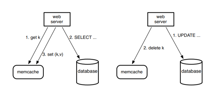
The assumption behind the architecture is that the user consumes much more content than they create. Thus using Memcached, which serves just like hashtable with CRUD operations, can serve as a building block and process billions of requests per second.

The basic workflow is that when a web server needs data, it first requests it on cache and if it is not cached, it will look for a SQL database. For write requests, a client will delete the key in Memcached, which puts the data in stale and then updates the database.[5]

However, such an architecture will introduce several fundamental problems:[6]

First, key-value cache is not a good semantic for graph operations. The look-ahead architecture will require the queries fetch the entire edge and changes to a single edge require the entire list to be reloaded because they deleted before. This is the bottleneck for concurrency performance. As in Facebook the connected components have thousands of connections on average and such an operation costs a lot of time and memory.

Second, visibility of updated data needs inter-regional communication because of the asynchronous master/slave replication for MySQL. The original model uses something called remote markers to track staled keys and asynchronously forward read from those keys to the master region. This needs a lot of inter-regional communication (just like walking from California to New York).

The Key to the Solution Is Modeling Data Through Graphs

Lacking Relationships Is the Key Failure of Other Kinds of Database Modeling [4]

Relational database works well if data is in codify paper forms and tabular structures. However, if we want to model the ad hoc relationships that will crop up in the real world, the RDBMS is poor at handling this.

As mentioned, the relational data model becomes a burden with a very large number of join tables, with sparsely populated rows where there are billions of different tables across databases. With the growth of such a dataset and the increased number of JOIN operations needed, the performance of existing RDBMS are no longer a fit for these business requirements.

Dealing with recursive queries such as the manager’s and employee’s report number will perform badly due to the computational and space complexity of recursively joining tables.

Nodes, Associations and Graph Modeling

So, it is true that traditional databases have implicit graph connections between different schemas. But as we analyze the semantic dependencies, such as A controls B, A buys B, as the data model defined, we need to check on the data table. We will see we are blind to these connections. If we want to make the connections visible before a check on the node, we need to define objects and their connections separately.

The key difference between graph databases and other databases is to represent nodes and paths separately. For example, we can represent people, or managers, as separate nodes. Associations capture the users’ friendships, belongings, authorship of the checkin and comments and the binding between the checkin and its location and comments.

We can add new nodes and new associations in a flexible way without compromising the existing network or migrating data (original data remains stateless). Based on this modeling technique, we can model the original social network problem in this way:

Here we can construct nodes and their corresponding paths separately and build a path as an association in an obvious way. Building the graph model in nGQL (a graph query language developed by Nebula Graph) can be followed as such: 

xxxxxxxxxx

-- Insert People

INSERT VERTEX person(ID, name) VALUES 1:(2020031601, ‘Jeff’);

INSERT VERTEX person(ID, name) VALUES 2:(2020031602, ‘A’);

INSERT VERTEX person(ID, name) VALUES 3:(2020031603, ‘B’);

INSERT VERTEX person(ID, name) VALUES 4:(2020031604, ‘C’);

-- Insert edge

INSERT EDGE manage (level_s, level_end) VALUES 1 -> 2: ('0'， '1')

INSERT EDGE manage (level_s, level_end) VALUES 1 -> 3: ('0'， '1')

INSERT EDGE manage (level_s, level_end) VALUES 1 -> 4: ('0'， '1')

And the query which we previously implemented with the extremely long SQL can be rewritten in a more concise way using Cypher or nGQL.

Here is the simple nGQL version:

xxxxxxxxxx

GO FROM 1 OVER manage YIELD manage.level_s as start_level, manage._dst AS personid

| GO FROM $personid OVER manage where manage.level_s < start_level + 3

YIELD SUM($$.person.id) AS TOTAL, $$.person.name AS list

And the Cypher version is in here: [1] 

xxxxxxxxxx

MATCH (boss)-[:MANAGES*0..3]->(sub),

(sub)-[:MANAGES*1..3]->(personid)

WHERE boss.name = “Jeff”

RETURN sub.name AS list, count(personid) AS Total

nGQL greatly reduced the query length which is essential for performance and debugging. For a comparison among Cypher, Gremlin and nGQL, refer to this post.

Why Graph Databases Have Better Performance

Graph databases have designed special optimizations for highly connected, unstructured data. Different kinds of graph databases have different implementations targeting different scenarios.

Here we will introduce several different kinds of graph databases, all of them natively support graph modeling.

Neo4j [4]

Neo4j is one of the best-known graph database, and widely adopted by well-known companies, such as by eBay, Microsoft and so on.

Native Graph Processing

A graph database has native processing capabilities if it exhibits a property called index-free adjacency. A database engine that utilizes index-free adjacency is one in which each node maintains direct reference to its adjacent nodes and each node will therefore act as a micro-index for other nearby nodes. This is much less taxing than using global indexes. It means that query times are independent of the total size of the graph and are instead simply proportional to the amount of the graph searched.

In simpler terms, index-lookups could be O(logN) in algorithmic complexity versus O(1) for lookup immediately from key-value relationship and traverse m steps. If we use an index approach, it costs O(mlogn) which only costs O(m) with an index-free adjacency solution.

As mentioned, relational databases perform poorly when we move away from modestly sized JOIN operations which mainly results from the number of index-lookups involved. In contrast to relational databases, where join-intensive query performance deteriorates as the dataset gets bigger, with a graph database performance tends to remain relatively constant, even as the dataset grows. This is because queries are localized to a portion of the graph.

In-Memory Cache

For Neo4j 2.2, it uses an LRU-K page cache. The page cache is an LRU-K page-affined cache, meaning the cache divides each store into discrete regions, and then holds a fixed number of regions per store file.

Pages are evicted from the cache based on a least frequently used (LFU) cache policy, nuanced by page popularity. That is, unpopular pages will be evicted from the cache in preference to popular pages, even if the latter have not been touched recently. This policy ensures a statistically optimal use of caching resources.

Janus Graph  [7]

Janus Graph itself does not focus on storage and analytics functionalities. The main purpose of this frame is to serve as a graph database engine which focuses on compact graph serialization, graph data modeling and efficient query execution.

Supporting robust modular interfaces for data persistence, data indexing and client access is the main purpose of this frame. It can be a useful solution for companies that just want to use graph modeling as their architecture solutions.

JanusGraph can use Cassandra, HBase and Berkeley DB as its storage adapter and use Elasticsearch, Solr or lucene for data indexing.

Broadly speaking, applications can interact with JanusGraph in two ways:

• Embed JanusGraph inside the application executing Gremlin queries directly against the graph within the same JVM. Query execution, JanusGraph’s caches, and transaction handling all happen in the same JVM as the application while data retrieval from the storage backend may be local or remote.

• Interact with a local or remote JanusGraph instances by submitting Gremlin queries to the server. JanusGraph natively supports the Gremlin Server component of the Apache TinkerPop stack.

Nebula Graph [8]

Here is listed several bird’s eye views on the system design of Nebula Graph, which is specially optimized for graph modeled data.

Key Value Store Graph Processing

Nebula Graph adopted vertexID + TagID as keys for local storage and it stores out-key and in-key separately in different locations. This supports O(k) look up and partitioning ensures high availability in a large distributed cluster.

In contrast to other storage designs, Nebula Graph natively supports distributed partitioning or sharding. This greatly increases the processing speed and fault tolerant capabilities.

Shared-Nothing Distributed Storage Layer

To help migrating data and provide a modular level storage engine it uses its own kv store library. Thus it supports storage service for a third party kv store such as HBase and so on.

Nebula Graph manages the distributed kv store in a unified scheduling way with meta service. All the partition distribution data and current machine status can be found in the meta service. Users can add or remove machines from a console and execute a balance plan. Plus, Multi-cluster Raft group with atomic CAS, and read-modify-write operations are fully used by raft serialization which enables immediate consistency.

Stateless Query Layer

In the query layer, nGQL will be paired to Abstract Syntax Tree and be converted to LLVM IR. The IR code can be passed to an execution planner for edge-level parallel execution and Just In Time execution. The complied query will be stored and if a user adopted the same query again, it will reuse the cached commands with no need for further parsing.

The Graph Database Is the Proven Trend

Graph databases have already attracted the attention of many analysts and consulting companies:

Graph analysis is possibly the single most effective competitive differentiator for organizations pursuing data-driven operations and decisions after the design of data capture. — Gartner

“Graph analysis is the true killer app for Big Data.” — Forrester

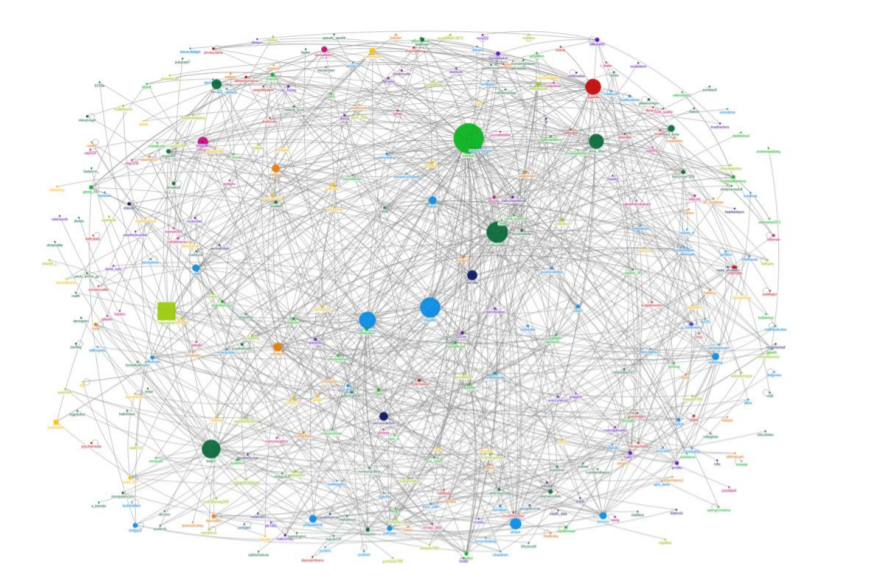
The current trend of graph database is the highest based on db-engine ranking:[9]

Graph Database With More Than Social Network

Netflix Cloud Database Engineering [10]:

Netflix adopted JanusGraph + cassandra + elasticsearch as their graph database infrastructure. The use of the graph database is in their digital asset management. Entities such as Assets, Movie, Display Sets and so on are vertex, and all relations are edges.

The current stats on this is that there are 200 million nodes in a PROD cluster. There are hundreds of queries and updates per minute, and 70 asset types and test clusters with over 200 million nodes too.

They also adopted a graph database in their authorization and distributed tracing. They also use it to visualize Netflix infra and relationships like how a code gets committed to a stash. It is built on jenkins and deployed by spinnaker.

Adobe [11]

There is a prejudice with new technologies that they may not suit large companies that may have many legacy systems. That it does not make sense to take the risk to change from an old stable system to a new and possibly unstable technology.

But Adobe did this with some transfer from an old NoSQL database to Neo4j.

The overhauling system’s name is Behance, which is a leading social media platform owned by Adobe and launched in 2005. It has more than 10 million members.

Here people can share their creative works with millions of daily visitors. 

Such a large legacy system was built upon MongoDB and Cassandra and, due to historical design problems, there were some daunting things to overcome.

MongoDB has very slow reads because of the data model and Cassandra, probably because of fan-out design policies and large overhead in web infrastructure. Plus, Cassandra needs babysitting by a huge number of ops team. As the original infra shows below, the fan-out to feed new project messages to followers needs a huge number of writes, which noticeably hampers performance:

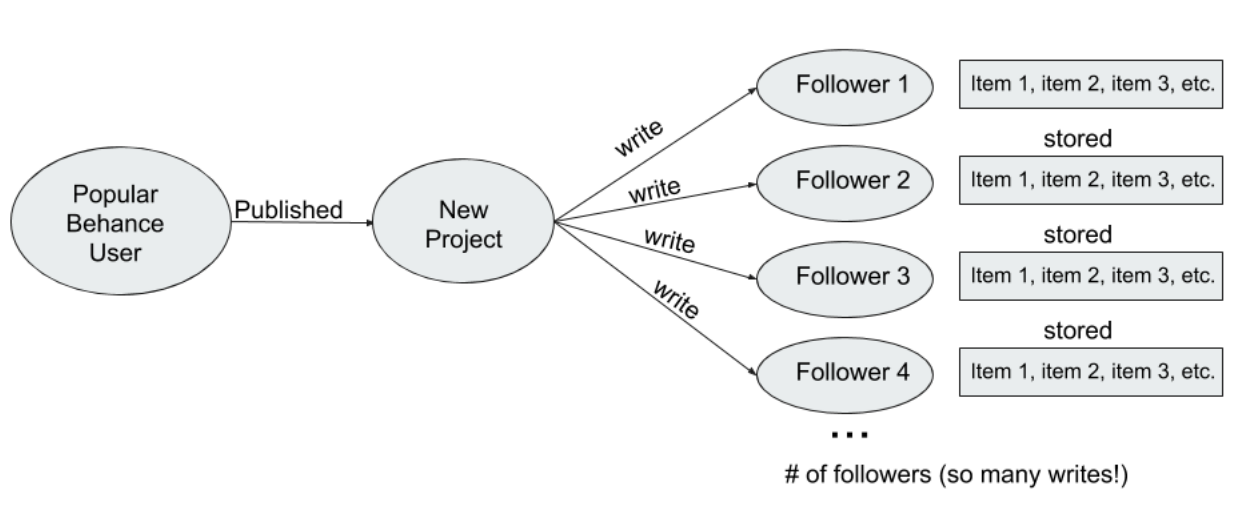
So, to have a flexible, efficient robust system with fast feed loading and minimal data storage, Adobe decided to migrate from the original Cassandra database to a Graph database with Neo4j.

The relationship here, separated one operation, such as appreciation, to different types of statuses, such as to enable a visit or not, and so on. These are named Tiered relationships. As a side note, such status information could be supported by Nebula Graph with just one edge.

Here is the data-model:

By adopting a simple leader-follower architecture, a huge performance gain was achieved: 

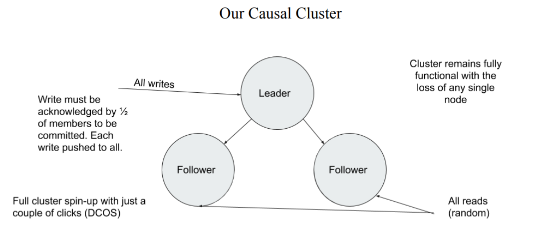
To be more specific, by adopting a graph database with a master-slave architecture for fault tolerance, the Adobe team acquired a huge number of performance improvements:[11]

1. Human maintenance hours down well over 300% with Neo4j
2. 1/1000 storage required - 50GB with Neo4j vs 50TB with Cassandra
3. Simple: powered by 3 instances instead of 48
4. Easy extensibility thanks to clean graph data model

Conclusion

Graph databases have many low hanging fruits for use in the big data era. Using graph databases as a technical solution are also ideal for other emerging technologies, like AI, IoT, 5G applications, and so on. But they can also transform legacy systems.

A graph database may have many different infrastructure implementations but they all support graph modeling which interconnect different components with their associations. As mentioned, such a sea of change in data modeling will be an extremely simple and straightforward solution for many daily system scenarios. They will also offer much faster throughput and lesser DevOps requirements.

References

[1] An Overview Of Neo4j And The Property Graph Model Berkeley, CS294, Nov 2015 https://people.eecs.berkeley.edu/~istoica/classes/cs294/15/notes/21-neo4j.pdf

[2] several original data sources from talk made by Duen Horng (Polo) Chau (Geogia tech) www.selectscience.net, www.phonedog.com, www.mediabistro.com, www.practicalecommerce.com/

[3] Graphs / Networks Basics, how to build & store graphs, laws, etc. Centrality, and algorithms you should know   Duen Horng (Polo) Chau(Georgia tech)

[4] Graph databases, 2nd Edition: New opportunities for Connected Data

[5] R. Nishtala, H. Fugal, S. Grimm, M. Kwiatkowski, H. Lee, H. C.Li, R. McElroy, M. Paleczny, D. Peek, P. Saab, D. Stafford, T. Tung, and V. Venkataramani. Scaling Memcache at Facebook. In Proceedings of the 10th USENIX conference on Networked Systems Design and Implementation, NSDI, 2013.

[6] Nathan Bronson, Zach Amsden, George Cabrera, Prasad Chakka, Peter Dimov Hui Ding, Jack Ferris, Anthony Giardullo, Sachin Kulkarni, Harry Li, Mark Marchukov Dmitri Petrov, Lovro Puzar, Yee Jiun Song, Venkat Venkataramani  TAO: Facebook’s Distributed Data Store for the Social Graph USENIX 2013

[7] Janus Graph Architecture https://docs.janusgraph.org/getting-started/architecture/

[8] Nebula Graph Architecture — A Bird’s View https://nebula-graph.io/posts/nebula-graph-architecture-overview/

[9] database engine trending https://db-engines.com/en/ranking_categories

[10] Netflix Content Data Management talk https://www.slideshare.net/RoopaTangirala/polyglot-persistence-netflix-cde-meetup-90955706#86

[11] Harnessing the Power of Neo4j for Overhauling Legacy Systems at Adobe https://neo4j.com/graphconnect-2018/session/overhauling-legacy-systems-adobe